aivis Engine v2 - Signal Monitor - User Guide
Download OpenAPI specification:Download
aivis Signal Monitor is one of the engines of the aivis Technology Platform by Vernaio.
aivis Signal Monitor monitors the health of the input signals and warns if a signal behaves in a way that is not observed from the historical data (or the training data).
Moreover, various characteristics are monitored for each signal, based not only on signal values but also on the signal update frequencies in the database.
The warning criteria, i.e., thresholds, for each characteristic are learned automatically and blazingly fast from the historical data.
aivis Signal Monitor acts as the first gatekeeper to ensure that any other data application is fed with high-quality data. But there is more to it:
data gatekeeper: are sensors and the data pipeline working as usual?
aivis Signal Monitor helps you noticing any problem in your data fast. Examples include broken sensors, misconfigurations, or delays in the data pipeline. This is an important task, as conform data are a prerequisite to any kind of further data application. Therefore, we recommend to run aivis Signal Monitor together with any aivis engine.
threshold monitoring: are all signal values within their allowed ranges?
Threshold monitoring is an integral part of condition monitoring. Typically, warnings are raised if certain signal values exceed thresholds that are defined either by the manufacturer or by some norm. For both cases, it is solely the users' responsibility to find "appropriate" thresholds. In contrast, aivis Signal Monitor learns thresholds from training. This allows users to include more signals and signal characteristics in the monitoring, while freeing them from the painstaking task of fine-tuning the threshold values. Note that, however, aivis Signal Monitor may lead to more restrictive thresholds, appearing more sensitive than standard threshold monitoring. Should there be a need to conform with manufacturer or standard thresholds, aivis Signal Monitor also allows triggering warnings by user-defined formulas.
anomaly detection: are there any deviations from the normal (production) process?
For the purpose of anomaly detection there is a dedicated engine: aivis Anomaly Detection. It is superior compared to aivis Signal Monitor as it can check complex relationships between many signals and is in general more sensitive to small deviations. However, aivis Signal Monitor is a perfect complement to the abilities of aivis Anomaly Detection. First, while you may want to monitor some processes more closely, a simpler approach might suffice for some other signals. Many anomalies become apparent already from looking at single signals. Second, with aivis Signal Monitor it is easier to monitor various signal characteristics. Each characteristic is monitored by a specific trigger. There are a few trigger types (see below) and more will be added in the future. Third, aivis Signal Monitor can help pin down immediately the source of any anomaly.
Some illustrative simple use cases are laid out below using the data of the getting started example. For more examples on aivis Signal Monitor and the other engines, please look at the general examples.
This documentation explains the usage and principles behind aivis Signal Monitor for data and software engineers. For detailed API descriptions of docker images, web endpoints and SDK functions, please consult the reference manual of the relevant component:
SDKs
- Python API reference: base, Signal Monitor.
- Java API reference.
- C API reference.
Docker Images
App-API
Web-API
For additional support, go to Vernaio Support.
Using aivis Signal Monitor consists of 2 steps:
- Training, which creates a prediction model based on the Training Data. The model can be thought of as a list of triggers each of which monitors a specific characteristic of a signal.
- Inference, which applies the model from the previous step to some Inference Data to monitor the inference data either for retrospective evaluation or live prediction.

Currently, aivis Signal Monitor is distributed to a closed user base only. To gain access to the artifacts, as well as for any other questions, you can open a support ticket via aivis Support.
The SDK of aivis Signal Monitor allows for direct calls from your C, Java or Python program code. All language SDKs internally use our native shared library (FFI). As C APIs can be called from various other languages as well, the C-SDK can also be used with languages such as R, Go, Julia, Rust, and more. Compared to the docker images, the SDK enables a more fine-grained usage and tighter integration.
In this chapter we will show you how to get started using the SDK.
A working sdk example that builds on the code explained below can be downloaded directly here:
- signal-monitor-examples.zip (latest)
For the following installation instruction, always replace:
{ENGINE}by the engine's acronym, heresmfor signal monitor{VERSION}by the aivis version you want to install, e.g.2.11.0{TARGET}by the target fitting your operating system, e.g.win_amd64- see artifacts for other options on linux and macosTo run aivis, there are two things you need in addition to the zipped examples you just downloaded: an aivis licensing key and access to Vernaio's artifact repository (Nexus Sonatype). To obtain them, please contact aivis Support.We recommend running the example in the following way:
- Make sure you have a valid Python (
>=3.10) installation. - Create an environment variable
AIVIS_ENGINE_V2_API_KEYand assign the aivis licensing key to it. - Make sure you have an active internet connection so that the licensing server can be contacted and dependencies can be downloaded.
- Download and unzip the examples from the link above. The folder now has the following structure:
+- data | +- # CSV file(s) containing the data the example is based on; Docker, Java and Python code read the same CSV files | +- docker | +- # files to run the example via Docker images which we won't need now | +- java | +- # files to run the example via Java SDK which we won't need now | +- python | +- # files to run the example via Python SDK - Navigate to the
**/pythonsubfolder. Here, you will find the classic.pyPython script and a.ipynbJupyter notebook. Both run the exact same example and output the same result. Choose which one you want to run. - Open a console in the
**/pythonsubfolder and run the following commands. - Make sure to install Poetry, a Python package manager:
python -m pip install poetry - Log in to Vernaio's artifact repository and (-> upper right) access your user token name code and user token pass code.
- Connect to the artifact repository:
# configure your credentials poetry config http-basic.vernaio-python <user token name code> <user token pass code> - Install aivis and other dependencies as defined in Poetry's configuration file
pyproject.toml. This step can take a little while:poetry install --no-root - Option A - run the classic Python script:
# runs the classic Python script `example_{ENGINE}.py` poetry run python example_{ENGINE}.py --input=../data --output=output - Option B - run the Jupyter notebook (the second command opens a tab in your browser):
# installs Jupyter kernel poetry run ipython kernel install --user --name=aivis # runs the Jupyter Python script `example_{ENGINE}.ipynb` poetry run jupyter notebook example_{ENGINE}.ipynb - After running the scripts, you will find your computation results in
**/python/output.
Done!!
Of course, there are various ways to install Python dependencies on your machine. We only mention some alternatives briefly here, as this is not specific to aivis and can be looked up everywhere. For example, you could download the dependencies as
.whlfiles from the artifact repository. You'll need the following ones, as also listed in Poetry's configuration filepyproject.toml:vernaio_aivis_engine_v2_{ENGINE}_runtime_python_full-{VERSION}-py3-none-{TARGET}.whl: A full Python runtime for the engine you want to runvernaio_aivis_engine_v2_base_sdk_python-{VERSION}-py3-none-any.whl: The base Python SDKvernaio_aivis_engine_v2_{ENGINE}_sdk_python-{VERSION}-py3-none-any.whl: The Python SDK for the engine you want to runvernaio_aivis_engine_v2_toolbox-{TOOLBOX-VERSION}-py3-none-any.whl: The toolbox Python SDK to post-process the output of aivis and generate an HTML report
These
.whlfiles can now be installed directly.You could still use Poetry and adapt the
pyproject.toml. (In that case, remove the vernaio-python source definition frompyproject.tomland skip thepoetry configstep from above.)[tool.poetry.dependencies] vernaio-aivis-engine-v2-base-sdk-python = { file = "path/to/vernaio_aivis_engine_v2_base_sdk_python-{VERSION}-py3-none-any.whl" } # etc.You are even free to ignore Poetry altogether and install the
.whlfiles directly in pip:pip install path/to/vernaio_aivis_engine_v2_base_sdk_python-{VERSION}-py3-none-any.whl # etc.Then you can directly run the Python script (don't forget
--input=../data --output=output) or the notebook in your preferred way.To run aivis, there are two things you need in addition to the zipped examples you just downloaded: an aivis licensing key and access to Vernaio's artifact repository (Nexus Sonatype). To obtain them, please contact aivis Support.Of course, there are various ways to install Java dependencies. We recommend running the example in the following way:
- Make sure you have a valid Java (
>=11) installation. - Create an environment variable
AIVIS_ENGINE_V2_API_KEYand assign the aivis licensing key to it. - Make sure you have an active internet connection so that the licensing server can be contacted.
- Download and unzip the examples from the link above. The folder now has the following structure:
+- data | +- # CSV file(s) containing the data the example is based on; Docker, Java and Python code read the same CSV files | +- docker | +- # files to run the example via Docker images which we won't need now | +- java | +- # files to run the example via Java SDK | +- python | +- # files to run the example via Python SDK which we won't need now - We use Gradle as our Java package manager. It's easiest to directly use the Gradle wrapper.
- Log in to Vernaio's artifact repository and (-> upper right) access your user token name code and user token pass code.
- Connect to the artifact repository by, e.g., adapting the
build.gradle:
(If you like, you could alternatively adapt yourcredentials { username <user token name code> password <user token pass code> }gradle.propertiesfile.) - Open a console in the
**/javasubfolder and run the following commands:# builds this Java project with Gradle wrapper ./gradlew clean build # runs Java with parameters referring to input and output folder java -jar build/libs/example_{ENGINE}.jar --input=../data --output=output - After running the scripts, you will find your computation results in
**/java/output.
Done!!
- Make sure you have a valid Python (
Our SDK artifacts come in two flavours:
fullpackages provide the full functionality and are available for mainstream targets only:win-x8664macos-armv8* (SDK >= 11.0) 2.3macos-x8664* (SDK >= 11.0; until aivis engine version 2.9.0) 2.3linux-x8664(glibc >= 2.14)
infpackages contain only API functions regarding the inference of a model. As lightweight artifacts they are available for a broader target audience:win-x8664macos-armv8* (SDK >= 11.0) 2.3macos-x8664* (SDK >= 11.0; until aivis engine version 2.9.0) 2.3linux-x8664(glibc >= 2.14)linux-armv7(glibc >= 2.18; until aivis engine version 2.9.0)linux-armv8(glibc >= 2.18; until aivis engine version 2.9.0)linux-ppc64(glibc >= 2.18; until aivis engine version 2.2.0)
* Only Python and C SDKs are supported. Java SDK is not available for this target.
In this chapter we want to demonstrate the full API functionality and thus always use the full package.
To use the Python-SDK you must download the SDK artifact (flavour and target generic) for your pythonpath at build time. Additionally at installation time, the runtime artifact must be downloaded with the right flavour and target.
The artifacts are distributed through a PyPI registry.
Using Poetry you can simply set a dependency on the artifacts specifying flavour and version. The target is chosen depending on your installation system:
aivis_engine_v2_sm_sdk_python = "{VERSION}"
aivis_engine_v2_sm_runtime_python_{FLAVOUR} = "{VERSION}"
The SDK supports the full API and will throw a runtime exception if a non-inference function is invoked with an inference-flavoured runtime.
To use the Java-SDK, you must download at build time:
- SDK artifact (flavour and target generic) for your compile and runtime classpath
- Runtime artifact with the right flavour and target for your runtime classpath
It is possible to include multiple runtime artifacts for different targets in your application to allow cross-platform usage. The SDK chooses the right runtime artifact at runtime.
The artifacts are distributed through a Maven registry.
Using Maven, you can simply set a dependency on the artifacts specifying flavour, version and target:
<dependency>
  <groupId>com.vernaio</groupId>
  <artifactId>aivis-engine-v2-sm-sdk-java</artifactId>
  <version>{VERSION}</version>
</dependency>
<dependency>
  <groupId>com.vernaio</groupId>
  <artifactId>aivis-engine-v2-sm-runtime-java-{FLAVOUR}-{TARGET}</artifactId>
  <version>{VERSION}</version>
  <scope>runtime</scope>
</dependency>
Alternativly, with Gradle:
implementation 'com.vernaio:aivis-engine-v2-sm-sdk-java:{VERSION}'
runtimeOnly    'com.vernaio:aivis-engine-v2-sm-runtime-java-{FLAVOUR}-{TARGET}:{VERSION}'
The SDK supports the full API and will throw a runtime exception if a non-inference function is invoked with an inference-flavoured runtime.
To use the C-SDK, you must download the SDK artifact at build time (flavour and target generic). For final linkage/execution you need the runtime artifact with the right flavour and target.
The artifacts are distributed through a Conan registry.
Using Conan, you can simply set a dependency on the artifact specifying flavour and version. The target is chosen depending on your build settings:
aivis-engine-v2-sm-sdk-c/{VERSION}
aivis-engine-v2-sm-runtime-c-{FLAVOUR}/{VERSION}
The SDK artifact contains:
- Headers:
include/aivis-engine-v2-sm-core-full.h
The runtime artifact contains:
- Import library (LIB file), if Windows target:
lib/aivis-engine-v2-sm-{FLAVOUR}-{TARGET}.lib - Runtime library (DLL file), if Windows target:
bin/aivis-engine-v2-sm-{FLAVOUR}-{TARGET}.dll(also containing the import library) - Runtime library (SO file), if Linux target:
lib/aivis-engine-v2-sm-{FLAVOUR}-{TARGET}.so(also containing the import library)
The runtime library must be shipped to the final execution system.
A valid licensing key is necessary for every aivis calculation in every engine and every component.
It has to be set (exported) as the environment variable AIVIS_ENGINE_V2_API_KEY.
aivis will send HTTPS requests to https://v3.aivis-engine-v2.vernaio-licensing.com (before release 2.7: https://v2.aivis-engine-v2.vernaio-licensing.com, before release 2.3: https://aivis-engine-v2.perfectpattern-licensing.de) to check if your licensing key is valid. Therefore, the requirements are an active internet connection as well as no firewall blocking an application other than the browser from calling this URL.
If aivis returns a licensing error, please check the following items before contacting aivis Support:
- Has the environment variable been set correctly?
- Licensing keys have the typical form
<FirstPartOfKey>.<SecondPartOfKey>with the first and second parts being UUIDs. In particular, there must be no whitespace. - Applications and, in particular, terminals often need to be restarted to learn newly set environment variables.
- Open
https://v3.aivis-engine-v2.vernaio-licensing.comin your browser. The expected outcome is "Method Not Allowed". In that case, at least the URL is not generally blocked. - Sometimes, firewalls block applications other than the browser from accessing certain or all websites. Try to investigate if you have such a strict firewall.
Before we can invoke API functions of our SDK, we need to set it up for proper usage and consider the following things.
Releasing Unused Objects
It is important to ensure the release of allocated memory for unused objects.
In Python, freeing objects and destroying engine resources like Data-, Training- and Inference-objects is done automatically. You can force resource destruction with the appropriate destroy function.
In Java, freeing objects is done automatically, but you need to destroy all engine resources like Data-, Training- and Inference-objects with the appropriate destroy function. As they all implement Java’s AutoClosable interface, we can also write a try-with-resource statement to auto-destroy them:
try(final SignalMonitorData trainingData = SignalMonitorData.create()) {

  // ... do stuff ...

} // auto-destroy when leaving block
In C, you must always
- free every non-null pointer allocated by the engine with aivis_free (all pointers returned by functions and all double pointers used as output function parameter e.g. Error*)
Note: aivis_free will only free own objects. Also, it will free objects only once and it disregards null pointers. - free your own objects with free as usual.
- destroy all handles after usage with the appropriate destroy function.
Error Handling
Errors and exceptions report what went wrong on a function call. They can be caught and processed by the outside.
In Python, an Exception is thrown and can be caught conveniently.
In Java, an AbstractAivisException is thrown and can be caught conveniently.
In C, every API function can write an error to the given output function parameter &err (to disable this, just set it to NULL). This parameter can then be checked by a helper function similar to the following:
const Error *err = NULL;

void check_err(const Error **err, const char *action) {

  // everything is fine, no error
  if (*err == NULL)
    return;

  // print information
  printf("\taivis Error: %s - %s\n", action, (*err)->json);

  // release error pointer
  aivis_free(*err);
  *err = NULL;

  // exit program
  exit(EXIT_FAILURE);
}
Failures within function calls will never affect the state of the engine.
Logging
The engine emits log messages to report on the progress of each task and to give valuable insights. These log messages can be caught via registered loggers.
# create logger
class Logger(EngineLogger):
    def log(self, level, thread, module, message):
        if (level <= 3):
            print("\t... %s" % message)

# register logger
SignalMonitorSetup.register_logger(Logger())
// create and register logger
SignalMonitorSetup.registerLogger(new EngineLogger() {

    public void log(int level, String thread, String module, String message) {
        if (level <= 3) {
            System.out.println(String.format("\t... %s", message));
        }
    }
});
// create logger
void logger(const uint8_t level, const char *thread, const char *module, const char *message) {
  if (lvl <= 3)
    printf("\t... %s\n", message);
}

// register logger
aivis_setup_register_logger(&logger, &err);
check_err(&err, "Register logger");
Thread Management
During the usage of the engine, a lot of calculations are done. Parallelism can drastically speed things up. Therefore, set the maximal threads to a limited number of CPU cores or set it to 0 to use all available cores (defaults to 0).
# init thread count
SignalMonitorSetup.init_thread_count(4)
// init thread count
SignalMonitorSetup.initThreadCount(4);
// init thread count
aivis_setup_init_thread_count(4, &err);
check_err(&err, "Init thread count");
Now that we are done setting up the SDK, we need to create a data store that holds our historical Training Data. In general, all data must always be provided through data stores. You can create as many as you want.
After the creation of the data store, you can fill it with signal data. The classic way to do it is writing your own reading function and adding signals, i.e. lists of data points, to the data context yourself, as it is shown in Data Reader Options.
We recommend using the built-in files reader, which processes a folder with CSV files that have to follow the CSV Format Specification.
We assume that the folder path/to/input/folder/ contains train_sm.csv.
# create empty data context for training data
training_data = SignalMonitorData.create()

# create config for files reader
files_reader_config = json.dumps(
    {
        "folder": "path/to/input/folder/"
    }
)

# read data
training_data.read_files(files_reader_config)

# ... use training data ...
// create empty data context for training data
try(final SignalMonitorData trainingData = SignalMonitorData.create()) {

  // create config for files reader
  final DtoTimeseriesFilesReaderConfig trainingFilesReaderConfig = new DtoTimeseriesFilesReaderConfig("path/to/input/folder/");

  // read data
  trainingData.readFiles(trainingFilesReaderConfig);

  // ... use training data ...

} // auto-destroy training data
// create empty data context for training data
TimeseriesDataHandle training_data = aivis_timeseries_data_create(&err);
check_err(&err, "Create training data context");

// create config for files reader
const char *reader_config = "{"
  "\"folder\": \"path_to_input_folder\""
"}";

// read data
aivis_timeseries_data_read_files(training_data, (uint8_t *) reader_config, strlen(reader_config), &err);
check_err(&err, "Read Files");

// ... use training data ...

// destroy data context
aivis_timeseries_data_destroy(training_data, &err);
check_err(&err, "Destroy data context");
training_data = 0;
In the following, we will assume you have read in the file train_sm.csv shipped with the example project.
With the data store filled with historical Training Data, we can now create our training:
# build training config
training_config = json.dumps({
        "triggers": [
            {"_type": "NumericalValueOutOfRange"},
            {"_type": "SignalInactive"},
        ],
        "signals": [
            {
                "signal": "SIGNAL_45",
                "interpreter": {"_type": "Categorical"},
                "additionalTriggers": [{"_type": "CategoricalValueUnknown"}],
            }
        ],
})

# create training and train the model
training = SignalMonitorTraining.create(training_data, training_config)

# ... use training ...
// build training config
final DtoSignalConfig[] signalConfigs =	{
  new DtoSignalConfig("SIGNAL_45").withInterpreter(new DtoCategoricalSignalInterpreter())
    .withAdditionalTriggers(new IDtoAbstractTriggerConfig[] { new DtoCategoricalValueUnknownTriggerConfig() }) };
final DtoTrainingConfig trainingConfig =
  new DtoTrainingConfig(new IDtoAbstractTriggerConfig[] { new DtoNumericalValueOutOfRangeTriggerConfig(), new DtoSignalInactiveTriggerConfig() })
    .withSignals(signalConfigs);

// create training and train the model
final SignalMonitorTraining training = SignalMonitorTraining.create(trainingData, trainingConfig) {

  // ... use training ...

} // auto-destroy training
// build training config
const char *training_config = "{"
    "\"triggers\": [{"
      "\"_type\": \"NumericalValueOutOfRange\""
    "},{"
      "\"_type\": \"SignalInactive\""
    "}],"
    "\"signals\": [{"
      "\"signal\": \"SIGNAL_45\","
      "\"interpreter\": {"
        "\"_type\": \"Categorical\""
      "},"
      "\"additionalTriggers\": [{"
        "\"_type\": \"CategoricalValueUnknown\""
      "}]"
    "}]"
"}";

// create training and train the model
SignalMonitorTrainingHandle training_handle = aivis_signal_monitor_training_create(
    training_data,
    (uint8_t *)training_config,
    strlen(training_config),
    &err);
check_err(&err, "Create training");

// ... use training ...

// destroy training
aivis_signal_monitor_training_destroy(training_handle, &err);
check_err(&err, "Destroy model");
training_handle = 0;
Notice that we are requesting two triggers, signal inactive and numerical value out of range for all signals.
Also note that SIGNAL_45 is interpreted as categorical and attach a categorical value unknown trigger.
For the moment, you may take this file as it is. The different keys will become clearer from the later sections and the reference manual.
As a next step, we create a second folder data and add the Training Data CSV file train_sm.csv to the folder. Afterwards, we create a blank folder output.
After the training has finished, we can evaluate it by running a historical evaluation (bulk inference) on the inference data (out-of-sample). This way, we obtain a continuous stream of values — exactly as it would be desired by the machine operator.
As we do the inference in the same process with the training, we can create the inference directly from the training. If these two processes were separated we could get the model explicitly from the training and write it to a file. The inference could then be created based on the content of the model file.
# build inference config
inference_config = json.dumps({})

# create inference
inference = SignalMonitorInference.create_by_training(training, inference_config)

# ... use inference ...
// build inference config
final DtoInferenceConfig inferenceConfig = new DtoInferenceConfig();

// create inference
try(final SignalMonitorInference inference = SignalMonitorInference.createByTraining(training, inferenceConfig)) {

  // ... use inference ...

} // auto-destroy inference
// build inference config
const char *inference_config = "{}";

// create inference
SignalMonitorInferenceHandle inference_handle = aivis_signal_monitor_inference_create_by_training_handle(
    training_handle,
    (uint8_t *)inference_config,
    strlen(inference_config),
    &err);
check_err(&err, "Create inference");

// ... use inference ...

// destroy inference
aivis_signal_monitor_inference_destroy(inference_handle, &err);
check_err(&err, "Destroy inference");
inference_handle = 0;
aivis Signal Monitor inference engine takes time ranges as an input. This list of time intervals defines the periods for which the signals are to be monitored by the inference engine.
# choose inference time ranges
time_ranges = json.dumps(
    {"timeRanges": [{"from": 1598918880000, "to": 1599094260000}]}
)

# produce warnings
inferences = inference.infer(inference_data, time_ranges)

# ... do something with warnings ...
// choose inference time ranges
final DtoInferenceTimeRanges timeRanges = new DtoInferenceTimeRanges(
  new DtoInferenceTimeRange [] {
    new DtoInferenceTimeRange(1598918880000L, 1599094260000L)
});

// produce warnings
final IDtoWarnings warnings = inference.infer(inferenceData, timeRanges);

// ... do something with warnings ...
// choose inference times ranges
const char *time_ranges = "{"
  "\"timeRanges\": [{"
    "\"from\": 1598918880000,"
    "\"to\": 1599094260000"
"}]}";

// produce warnings
const char *warnings = aivis_signal_monitor_inference_infer(
    inference_handle,
    inference_data,
    (uint8_t *)time_ranges,
    strlen(time_ranges),
    &err);
check_err(&err, "Infer warnings");

// ... do something with warnings ...

// free warnings
aivis_free(warnings);
warnings = NULL;

// destroy inference
aivis_signal_monitor_inference_destroy(inference_handle, &err);
check_err(&err, "Destroy inference");
inference_handle = 0;
Results of this inference are discussed below. But first, we will do the same calculations with docker images.
The docker images of aivis Signal Monitor are prepared for easy usage. They use the SDK internally but have a simpler file-based interface. If you have a working docker workflow system like Argo, you can build your own automated workflow based on these images.
In this chapter, we will show you how to get started using docker images.
A working example that builds on the code explained below can be downloaded directly here: signal-monitor-examples.zip.
This zip file contains example code for docker, python and java in respective subfolders. All of them use the same dataset which is in the data subfolder.
Prerequisites: Additionally to the signal-monitor-examples.zip you just downloaded, you need the following artifacts. To gain access, you can open a support ticket via aivis Support.
- The docker images
aivis-engine-v2-sm-training-worker,aivis-engine-v2-sm-inference-workerand (optionally for HTML report generation)aivis-engine-v2-toolbox - An aivis licensing key, see licensing
As a Kubernetes user even without deeper Argo knowledge, the aivis-engine-v2-example-sm-argo.yaml shows best how the containers are executed after each other, how training and inference workers are provided with folders that contain the data CSVs and how the toolbox assembles an HTML report at the end.
There are 3 different docker images:
- The Training Worker creates the model:
docker-releases.artifacts.vernaio.com/vernaio/aivis-engine-v2-sm-training-worker:{VERSION} - The Inference Worker creates predictions for a predefined time window in a bulk manner. This is convenient for evaluating a model:
docker-releases.artifacts.vernaio.com/vernaio/aivis-engine-v2-sm-inference-worker:{VERSION} - The Inference Service offers a RESTful web API that allows the triggering of individual predictions for a specified time via an HTTP call:
docker-releases.artifacts.vernaio.com/vernaio/aivis-engine-v2-sm-inference-service:{VERSION}
All docker images are Linux-based.
You need an installation of Docker on your machine as well as access to Vernaio's artifact repository. Log in to Vernaio's artifact repository and (-> upper right) access your user token name code and user token pass code.
docker -v
docker login docker-releases.artifacts.vernaio.com <user token name code> <user token pass code>
docker pull docker-releases.artifacts.vernaio.com/vernaio/aivis-engine-v2-sm-training-worker:{VERSION}
docker -v
docker login docker-releases.artifacts.vernaio.com <user token name code> <user token pass code>
docker pull docker-releases.artifacts.vernaio.com/vernaio/aivis-engine-v2-sm-training-worker:{VERSION}
A valid licensing key is necessary for every aivis calculation in every engine and every component.
It has to be set (exported) as the environment variable AIVIS_ENGINE_V2_API_KEY.
aivis will send HTTPS requests to https://v3.aivis-engine-v2.vernaio-licensing.com (before release 2.7: https://v2.aivis-engine-v2.vernaio-licensing.com, before release 2.3: https://aivis-engine-v2.perfectpattern-licensing.de) to check if your licensing key is valid. Therefore, the requirements are an active internet connection as well as no firewall blocking an application other than the browser from calling this URL.
If aivis returns a licensing error, please check the following items before contacting aivis Support:
- Has the environment variable been set correctly?
- Licensing keys have the typical form
<FirstPartOfKey>.<SecondPartOfKey>with the first and second parts being UUIDs. In particular, there must be no whitespace. - Applications and, in particular, terminals often need to be restarted to learn newly set environment variables.
- Open
https://v3.aivis-engine-v2.vernaio-licensing.comin your browser. The expected outcome is "Method Not Allowed". In that case, at least the URL is not generally blocked. - Sometimes, firewalls block applications other than the browser from accessing certain or all websites. Try to investigate if you have such a strict firewall.
First, we need to train the model (workflow step 1: Training) using the Training Worker.
At the beginning, we create a folder docker, a subfolder training-config and add the configuration file config.yaml:
data:
  folder: /srv/data
  dataTypes:
    defaultType: FLOAT
training:
  trainingConfig:
    triggers:
      - _type: SignalInactive
      - _type: NumericalValueOutOfRange
    signals:
      - signal: SIGNAL_45
        interpreter: Categorical
        additionalTriggers:
          - _type: CategoricalValueUnknown
output:
  folder: /srv/output
Notice that we are requesting two triggers, signal inactive and numerical value out of range for all signals.
Also note that SIGNAL_45 is interpreted as categorical and attach a categorical value unknown trigger.
For the moment, you may take this file as it is. The different keys will become clearer from the later sections and the docker reference manual.
As a next step, we create a second folder data and add the Training Data CSV file train_sm.csv to the folder. Afterwards, we create a blank folder output.
Our folder structure should now look like this:
+- docker
|  +- training-config
|      +- config.yaml
|
+- data
|  +- train_sm.csv
|
+- output
Finally, we can start our training via:
docker run --rm -it \
  -v $(pwd)/docker/training-config:/srv/conf \
  -v $(pwd)/data/train_sm.csv:/srv/data/train_sm.csv \
  -v $(pwd)/output:/srv/output \
  -e AIVIS_ENGINE_V2_API_KEY={LICENSE_KEY} \
  docker-releases.artifacts.vernaio.com/vernaio/aivis-engine-v2-sm-training-worker:{VERSION}
docker run --rm -it `
  -v ${PWD}/docker/training-config:/srv/conf `
  -v ${PWD}/data/train_sm.csv:/srv/data/train_sm.csv `
  -v ${PWD}/output:/srv/output `
  -e AIVIS_ENGINE_V2_API_KEY={LICENSE_KEY} `
  docker-releases.artifacts.vernaio.com/vernaio/aivis-engine-v2-sm-training-worker:{VERSION}
After a short time, this should lead to an output file model.json in the output folder.
It holds all model information for the following Inference.
After the training has finished, we can evaluate it by running a historical evaluation (bulk inference) on the second data file. This is the out-of-sample evaluation.
For this, we create a second subfolder inference-config of the docker folder and add the configuration file config.yaml:
data:
  folder: /srv/data
  dataTypes:
    defaultType: FLOAT
inference:
  config:
    dataFilter:
  modelFile: /srv/output/model.json
  timeRanges:
    - from: 1598918880000
      to: 1599094260000
output:
  folder: /srv/output
aivis Signal Monitor inference engine takes time ranges as an input. This list of time intervals defines the periods for which the signals are to be monitored by the inference engine.
After that, we add the Inference Data CSV file eval_sm.csv to the data folder.
Our folder structure should now look like this:
+- docker
|  +- training-config
|      +- config.yaml
|  +- inference-config
|      +- config.yaml
|
+- data
|  +- train_sm.csv
|  +- eval_sm.csv
|
+- output
|  +- model.json
Finally, we can run the Inference via:
docker run --rm -it \
  -v $(pwd)/docker/inference-config:/srv/conf \
  -v $(pwd)/data/eval_sm.csv:/srv/data/eval_sm.csv \
  -v $(pwd)/output:/srv/output \
  -e AIVIS_ENGINE_V2_API_KEY={LICENSE_KEY} \
  docker-releases.artifacts.vernaio.com/vernaio/aivis-engine-v2-sm-inference-worker:{VERSION}
docker run --rm -it `
  -v ${PWD}/docker/inference-config:/srv/conf `
  -v ${PWD}/data/eval_sm.csv:/srv/data/eval_sm.csv `
  -v ${PWD}/output:/srv/output `
  -e AIVIS_ENGINE_V2_API_KEY={LICENSE_KEY} `
  docker-releases.artifacts.vernaio.com/vernaio/aivis-engine-v2-sm-inference-worker:{VERSION}
Successful execution should lead to the file warnings.json in the output folder, which holds warnings.
At this stage, we would like to show some use cases for aivis Signal Monitor, without going into too much detail of terminologies and methodology of the engine.
Signal Inactive
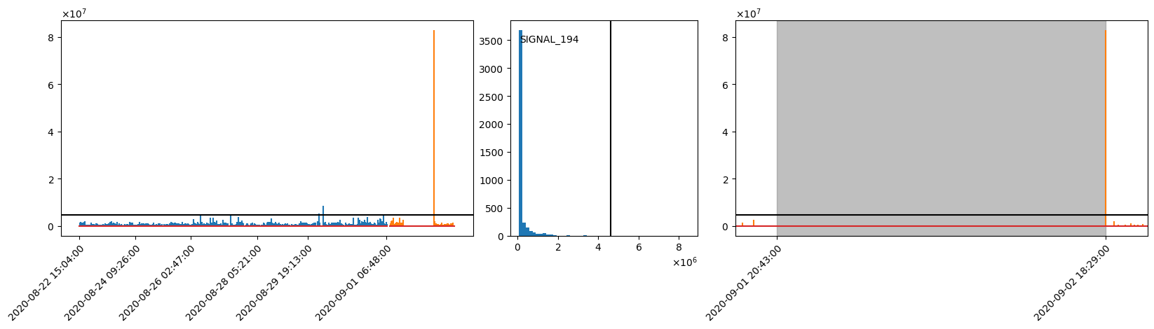
During the live inference phase of any predictive engine, e.g., aivis Signal Prediction, it is crucial to ensure the relevant signals are being updated at the same frequency as was observed in the training period. When such signals are not arriving in time, the quality of the prediction degrades over time.
Here, in this example, SIGNAL_194 was outputting signals at a healthy frequency, but suddenly it stopped working for a whole day. It seems the sensor might have been compromised, and it took some time to find the problem and fix/replace the sensor. During the disruption, SIGNAL_194 didn't output any new data, resulting in sub-optimal prediction quality.
aivis Signal Monitor can successfully detect such a disruption and notify users as soon as possible via a signal inactive trigger. The users can quickly learn what's going wrong and address the problem before the disruption becomes too costly.
Visualization
Left: Timeseries plot of training (blue) and out-of-sample inference data (orange).
Height of the vertical lines indicates the time difference between two adjacent data points.
A high value thus means that SIGNAL_194 has not been updated for a long time.
The black horizontal line indicates the threshold for the signal inactive trigger.
Center: Histogram of the time differences in the training data. Again, the black vertical line indicates the threshold.
Right: Zoomed in view of the inference timeseries where the warning is raised.
The grey area indicates the beginning and the end of the warning.
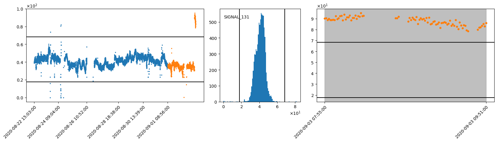
Numerical Value Out Of Range
Suppose we are running the aivis Anomaly Detection engine. During the inference, we notice a sudden increase in the anomaly score.
As aivis Signal Monitor is running in parallel, the cause of this sudden increase becomes evident immediately.
Simultaneously with the sudden increase in the anomaly score, the signal monitor raises a warning for SIGNAL_131.
It turns out that from 03.09.2020 on, the unit of SIGNAL_131 has been changed from Celsius to Fahrenheit, causing a sudden and huge jump in the signal values.
The numerical value out of range trigger can be helpful in detecting such odd behaviors in signals, allowing users to ensure good prediction quality of other engines.
Visualization
Left: Timeseries plot of training (blue) and out-of-sample inference data (orange).
The black horizontal lines indicate the upper and lower thresholds for the numerical value out of range trigger .
Center: Histogram of the training data. The black vertical lines indicate the upper and lower thresholds.
Right: Zoomed in view of the inference timeseries where the warning is raised.
The gray area is defined by the beginning and the end of the warning.
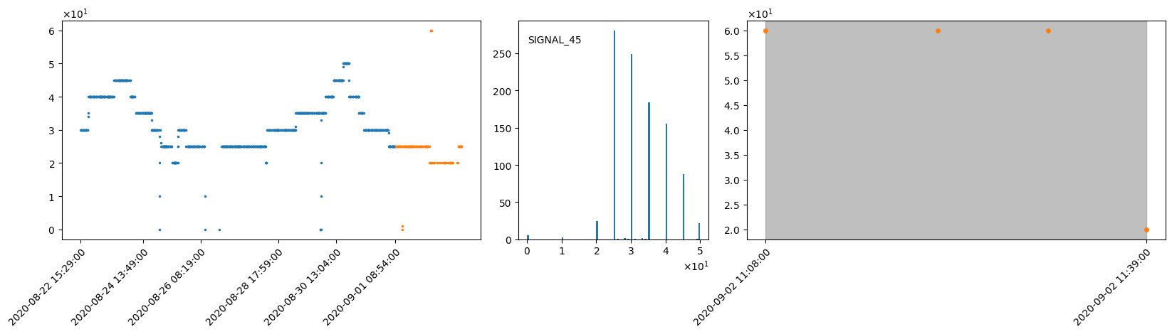
Categorical Value Unknown
aivis Signal Monitor can also detect and warn about a categorical signal outputting unknown category values via a categorical value unknown trigger.
SIGNAL_45 is a categorical signal, and during the training, the engine learned that this signal has 9 categories [0, 10, 20, 25, 30, 35, 40, 45, 50]. However, during out-of-sample inference, a new (unknown) category appears: category 60.
Visualization
Left: Timeseries plot of training (blue) and out-of-sample inference data (orange).
Center: Histogram of the training data.
Right: Zoomed in view of the inference timeseries where the warning is raised.
The gray area is defined by the beginning and the end of the warning of the categorical value unknown trigger .
In the next chapter we will focus on the nature of input data.
In the course of using aivis, large amounts of data are ingested. This chapter explains the terminology as well as the required format, quality, and quantity.
Most aivis engines work on time series data that is made up of signals. Every signal consists of two things, these being
- an ID, which is any arbitrary String except
timestampandavailability. The ID needs to be unique within the data. - a list of data points. Each data point consists of a signal value and a specific point in time, the Detection Timestamp (optionally there can also be an Availability Timestamp, but more on that later). Usually the values are the result of a measurement taken by a physical sensor like a thermometer, photocell, or electroscope, but you can also use market KPIs like stock indices or resource prices as a signal.
The data points for one or more signals for a certain detection time range are called a history.

The values of a signal can be boolean values, 64-bit Floating Point numbers or Strings. Non-finite numbers (NAN and infinity) and empty strings are regarded as being unknown and are therefore skipped.
Points in time are represented by UNIX Timestamps in milliseconds (64-bit Integer). This means the number of milliseconds that have passed since 01.01.1970 00:00:00 UTC.
Detection Timestamp
The point in time that a signal value belongs to is called the Detection Timestamp. This is usually the timestamp when the measurement originally took place. If the measurement is a longer offline process, it should refer to the point in time at which the measured property was established, e.g., the time point of sample drawing or the production time for delayed sampling. In case of the target signal, the Detection Timestamp should be set to the time you would have liked to have measured the signal online. In the aivis Signal Prediction example use case, the paper quality is such a signal. It is measured around 2 hours after the production of the paper in a laboratory and must be backdated to a fictitious, but instantaneous quality measurement in the process.
Different signals may have different Detection Timestamps. Some might have a new value every second, some every minute, some just when a certain event happens. aivis automates the process of synchronizing them internally. This includes dealing with holes in the data.
Availability Timestamp
When doing a historical evaluation, we want to know what the engine would have inferred/predicted for a list of Inference Timestamps that lie in the past (Inference Timestamps are the moments for which you want to get an inference). For a realistic inference, the engine must ignore all signal values that were not yet available to the database at the Inference Timestamp. A good example of such a case is a measurement that is recorded by a human. The value of this measurement will be backdated by him/her to the Detection Timestamp, but it took e.g., 5 minutes to extract the value and report it to the system. So, it would be wrong to assume that one minute after this fictitious Detection Timestamp, the value would have already been available to the Inference. Another example case is the fully automated lagged data ingestion of distributed systems (especially cloud systems).
There are multiple ways to handle availability. Which strategy you use depends on the concrete use case.

To allow for these different strategies, every data point can have an additional Availability Timestamp that tells the system when this value became available or would have been available. Signal values for which the Availability Timestamp lies after the Inference Timestamp are not taken into account for an inference at this Inference Timestamp.
If there is no knowledge about when data became available, the Availability Timestamp can be set to the Detection Timestamp — but then you must keep in mind that your historical evaluation might look better than it could have been in reality.
aivis works best on raw, unprocessed data. It is important to keep the following rules in mind:
- Remove signals beforehand only if you are absolutely sure that they are unrelated to your objective! The engine will select all relevant signals, anyway, and removing signals may reduce quality.
- Avoid linear interpolation (or similar data processing steps), as this would include information from the future and therefore invalidate or worsen the results.
- It is okay (except for aivis Signal Monitor) to drop consecutive duplicate values of one signal (e.g., if the value stays the same for a long period of time). This is because the engine assumes the value of a signal to be constant until a new data point is given, though there are subtleties for the target signal. It is, however, not advisable to drop duplicate values when running aivis Signal Monitor
SignalInactivetrigger, since the engine learns how often the signal gets new data points. - Do not train the engine on signals that wouldn't be there in live operation (i.e., during the inference phase). Doing so could harm the prediction quality because the engine might choose to use these soon-to-be-missing signals for prediction. For aivis Signal Monitor, this may produce unnecessary (or false) warnings (e.g.,
SignalInactive).
There is the possibility of filtering the Training Data in multiple ways:
- The overall time window can be restricted.
- Signals can be excluded and included as a whole.
- Specific time windows of specific signals can be excluded or included.
The filtering is configurable:
- The docker image Training Worker can be configured in the main config file.
- SDK Training API has filter nodes in the their config structure.
This means that two models could be trained on the same data set, but on different time windows or signal sets. Alternatively, the user can of course also restrict the data that enters the engine beforehand.
aivis uses data at two distinct points in the workflow:
- Training Data is used to train a model from knowledge that was derived from historical data. To ensure high quality of the model, you should use as many signals as possible over a period of time in a fine resolution that fits to your objective. The engine can ingest several thousands of signals and time ranges over multiple years. The idea is to simply put in all the data you have. The engine will filter out irrelevant signals by itself.
- Inference Data is the small amount of live data that is used as the direct input to make an inference/prediction. For each Inference Timestamp, the engine needs a small and recent history of the relevant signals to understand the current situation of the system. You can find more information on this in the next section Inference Data Specification.
When making an inference, aivis must know the current state of the real system by including a small portion of history.
In Training, the engine calculates which signals among the many signals in the Training Data will be relevant for the Inference. Furthermore, for each relevant signal, a time window is specified relative to the Inference Timestamp. This time window determines which values of the signal must be included in order to make a prediction for said timestamp. This doesn't only include the values within the time window but also either the value right at the start or the last value before the time window (see "Nearest Predecessor"). This information is called the Inference Data Specification and must be obeyed strictly when triggering Inference, as the engine relies on this data.
You can inspect a model for its Inference Data Specification.
It is possible to set the maximum amount of time to be included in the local history. This is done in the configuration of the Training via the parameter Maximal Lag.
The following diagram gives you a visual representation of how an Inference Data Specification could look like:

In the diagram you see that a start lag and end lag is specified for every signal. For the Inference, this means that for each signal we need all data points whose detection timestamps lie in the window [ inference timestamp - start lag; inference timestamp - end lag ] as well as the nearest predecessor (see below).
Nearest Predecessor
As previously mentioned, it is essential that you provide data for the whole time window. Especially, it must be clear what the value at the beginning is, i.e., at inference timestamp - start lag.
Typically, there is no measurement for exactly this point in time. Then, you must provide the nearest predecessor. This is the last value before the beginning of the time window. Then, the engine can at least take this value as an estimate. Of course, this first data point must also be available at the Inference Timestamp (regarding the Availability Timestamp).

Depending on the configuration, the engine will either throw an error or ignore timestamps for which you provide neither a value at the beginning of the time window nor a nearest predecessor. This implies that you always need at least one available value per relevant signal. Sending more data outside the demanded time window will have no effect on the inference.
Use built-in files reader (Docker)
For docker users, the only option to read data is providing data files following the CSV Format Specification, which are processed by the built-in files reader.
Use built-in files reader (SDK)
Since 2.10, SDK users also have the option to use the built-in files reader, which we recommend: The reader has been highly optimized and is e.g., capable of deterministic parallel reading. It is also equipped with various filtering options, so that unneeded data is not even added to the data context, which saves memory.
We assume that the folder path/to/input/folder/ contains CSVs following the CSV Format Specification. Two of them (with the ID product_type and color) are string signals, which have to be explicitly listed in the file reader's config, since the default is to assume all signal types are float.
# create empty data context, replace <<Engine>> by the engine you're using
data_context = <<Engine>>Data.create()

# create config for files reader
files_reader_config = json.dumps(
    {
        "folder": "path/to/input/folder/",
        "dataTypes": {
           "stringSignals": ["product_type", "color"]
        }
    }
)

# read data
data_context.read_files(files_reader_config)
// create empty data context, replace <<Engine>> by the engine you're using
try(final <<Engine>>Data dataContext = <<Engine>>Data.create()) {

  // create config for files reader
  final DtoTimeseriesFilesReaderConfig filesReaderConfig = new DtoTimeseriesFilesReaderConfig("path/to/input/folder/")
      .withDataTypes(new DtoTimeseriesDataTypesConfig().withStringSignals({"product_type", "color"}));

  // read data
  dataContext.readFiles(filesReaderConfig);

} // auto-destroy data
// create empty data context
TimeseriesDataHandle data_context = aivis_timeseries_data_create(&err);
check_err(&err, "Create data context");

// create config for files reader
const char *reader_config = "{"
  "\"folder\": \"path_to_input_folder\"",
  "\"dataTypes"\: {"
      "\"stringSignals\": [\"product_type\", \"color\"]"
   "}"
"}";

// read data
aivis_timeseries_data_read_files(data_context, (uint8_t *) reader_config, strlen(reader_config), &err);
check_err(&err, "Read Files");

// ... use data ...

// destroy data context
aivis_timeseries_data_destroy(data_context, &err);
check_err(&err, "Destroy data context");
data_context = 0;
Create your own reader (SDK)
You can directly process any data source of your choice by writing your own reader. You build data points and add them to the data context, which looks like this:
# create empty data context, replace <<Engine>> by the engine you're using
data_context = <<Engine>>Data.create()

# add sample data
data_context.add_float_signal("signal-id", [
  DtoFloatDataPoint(100, 1.0),
  DtoFloatDataPoint(200, 2.0),
  DtoFloatDataPoint(300, 4.0),
])

# ... use data context ...
// create empty data context, replace <<Engine>> by the engine you're using
try(final <<Engine>>Data dataContext = <<Engine>>Data.create()) {

  // add sample data
  dataContext.addFloatSignal("signal-id", Arrays.asList(
    new DtoFloatDataPoint(100L, 1.0),
    new DtoFloatDataPoint(200L, 2.0),
    new DtoFloatDataPoint(300L, 3.0),
  ));

  // ... use data context ...

} // auto-destroy data context
// create empty data context
TimeseriesDataHandle data_context = aivis_timeseries_data_create(&err);
check_err(&err, "Create data context");

const DtoFloatDataPoint points[] = {
  {100, 1.0},
  {200, 2.0},
  {300, 4.0},
};

// add sample data
aivis_timeseries_data_add_float_signal(data_context, "signal-id", &points[0], sizeof points / sizeof *points, &err);
check_err(&err, "Adding signal");

// ... use data context  ...

// destroy data context
aivis_timeseries_data_destroy(data_context, &err);
check_err(&err, "Destroy data context");
data_context = 0;
Above we have filled the data store with three hard-coded data points to illustrate the approach. Usually you will read in the data from some other source with your own reading function.
Please also note that the data reading is the place where decisions about signal data types are made. The code above obviously adds a float signal, which is analogous for the other data types.
All artifacts (SDKs and docker images) have a built-in data reader which can process CSV files. As the CSV format is highly non-standardized, we will discuss it briefly in this section.
CSV files must be stored in a single folder specified in the config under data.folder. Within this folder the CSV files can reside in an arbitrary subfolder hierarchy. In some cases (e.g. for HTTP requests), the folder must be passed as a ZIP file.
General CSV rules:
- The file's charset must be UTF-8.
- Records must be separated by Windows or Unix line ending (
CR LF/LF). In other words, each record must be on its own line. - Fields must be separated by commas.
- The first line of each CSV file represents the header, which must contain column headers that are file-unique.
- Every record including the header must have the same number of fields.
- Text values must be enclosed in quotation marks if they contain literal line endings, commas, or quotation marks.
- Quotation marks inside such a text value have to be prefixed (escaped) with another quotation mark.
Special rules:
- One column must be called
timestampand contain the Detection Timestamp as UNIX Timestamps in milliseconds (64-bit Integer) - Another column can be present that is called
availability. This contains the Availability Timestamp in the same format as the Detection Timestamp. - All other columns, i.e., the ones that are not called
timestamporavailability, are interpreted as signals. - Signal IDs are defined by their column headers
- If there are multiple files containing the same column header, this data is regarded as belonging to the same signal
- Signal values can be boolean values, numbers, and strings
- Empty values are regarded as being unknown and are therefore skipped
- Files directly in the data folder or in one of its subfolders are ordered by their full path (incl. filename) and read in this order
- If there are multiple rows with the same Detection Timestamp, the data reader proceeds all to the engine, which uses the last value that has been read
Boolean Format
Boolean values must be written in one of the following ways:
true/false(case insensitive)1/01.0/0.0with an arbitrary number of additional zeros at the end
Regular expression: (?i:true)|(?i:false)|1(\.0+)?|0(\.0+)?
Number Format
Numbers are stored as 64-bit Floating Point numbers. They are written in scientific notation like -341.4333e-44, so they consist of the compulsory part Significand and an optional part Exponent that is separated by an e or E.
The Significand contains one or multiple figures and optionally a decimal separator .. In such a case, figures before or after the separator can be omitted and are assumed to be 0. It can be prefixed with a sign (+ or -).
The Exponent contains one or multiple figures and can be prefixed with a sign, too.
The 64-bit Floating Point specification also allows for 3 non-finite values (not a number, positive infinity and negative infinity) that can be written as nan, inf/+inf and -inf (case insensitive). These values are valid, but the engine regards them as being unknown and they are therefore skipped.
Regular expression: (?i:nan)|[+-]?(?i:inf)|[+-]?(?:\d+\.?|\d*\.\d+)(?:[Ee][+-]?\d+)?
String Format
String values must be encoded as UTF-8. Empty strings are regarded as being unknown values and are therefore skipped.
Example
timestamp,availability,SIGNAL_1,SIGNAL_2,SIGNAL_3,SIGNAL_4,SIGNAL_5
1580511660000,1580511661000,99.98,74.33,1.94,true,
1580511720000,1580511721000,95.48,71.87,-1.23,false,MODE A
1580511780000,1580511781000,100.54,81.19,,1e-5,MODE A
1580511840000,1580511841000,76.48,90.01,2.46,0.0,MODE C
...
Previous sections gave an introduction on how to use aivis Signal Monitor and also shed some light on how it works. The following sections will explain more about the concept and provide a more profound background. It is not necessary to know this background to use aivis Signal Monitor! However, you may find convenient solutions for specific problems, or information on how to optimize your usage of aivis Signal Monitor. The following sections are organized in the natural order of the workflow. By workflow, we mean the cycle of data preparation, model training, finally utilizing it by making inferences, and continuous improvements. It will become clear that only minimal user input is required for this workflow. Nevertheless, the user has the option to control the process with several input parameters which will be presented below.
To train aivis Signal Monitor only minimal preparation is required, but of course, you need some dataset. The dataset should be representative of your application. For example, if you want to be warned if some sensor or machine is down, downtimes need to be excluded from the training. To achieve tight thresholds, it is often advisable to exclude maintenance periods. If there was any period of misbehavior, you likely also want to exclude that period. In the training, an automatic outlier exclusion is applied. This relieves you from the task of finding any short deviation from the normal process. However, it is assumed that at least 99% of each signal's data points are clean. Therefore, some exclusions are often necessary, and a convenient way is via the operative periods. On the other hand, data can also be non-representative because they do not cover all relevant states. For example, when the machines were run always with the same fixed speed during the training period, then switching this speed will raise warnings in inference. To avoid the unwanted warnings, the training period should include data for different speeds. However, because this is not always possible, there is also the possibility to adjust the model after training, see below.
Based on some user configuration, the signal monitor model is trained automatically from the training data. The model consists of a set of triggers, each defining a condition to raise a warning. As triggers are central to aivis Signal Monitor, below we will start by presenting the available triggers. Next, training configuration options will be explained. Here we focus on explaining the underlying concepts. When it comes to actually making the inputs, syntactical questions will be answered by the aivis reference manuals, which define the exact inputs that can be made depending on whether you are using one of the SDKs or a Docker container.
Different triggers monitor different characteristics of different, or even of the same signal. Below, all available trigger types are listed and explained. Note, however, that more trigger types are planned for the near future.
Signal Inactive
A signal inactive trigger raises a warning if the monitored signal does not output (update) a new data point within some maximum allowed update period. An update period is the difference in timestamps between two consecutive data points. The threshold below which update periods are still allowed, is learned from the training data.
There is only one parameter, sensitivity, to configure the training.
It is optional and controls how sensitive the trigger should be.
The higher the sensitivity, the more warnings will be raised;
a sensitivity of 0 means that the trigger will not produce any warning.
This trigger can work on any interpreter.
Numerical Value Out Of Range
A numerical value out of range trigger raises a warning if the monitored signal outputs a value that is out of the normal range. The normal range is defined by an upper threshold and a lower threshold. These thresholds are learned from the training data.
Again, there is only one parameter, sensitivity, to configure the training.
It is optional and controls how sensitive the trigger should be.
The higher the sensitivity, the more warnings will be raised;
a sensitivity of 0 means that the trigger will not produce any warning.
This trigger works only on signals with numerical interpreter.
Numerical Linear Relation Broken
2.8
A numerical linear relation broken trigger raises a warning if the monitored signal outputs a value that deviates from a linear model prediction. The linear model is defined by
- the target (the signal predicted),
- a set of predictor signals and associated slopes (the linear model coefficients),
- the intercept (the constant term of the linear model) and
- the threshold (the maximal allowed deviation between prediction and observation).
There are three optional parameters to configure the training of this trigger.
The maximal dimension sets the maximal number of predictor signals in a trigger's linear model.
On the one hand, the more signals a linear model contains, the more complex relationships can be monitored.
On the other hand, the triggers' warnings may be more difficult to interpret for linear models that contain many signals.
Moreover, training of this trigger can take noticeable computing time and this increases with the maximal dimension.
By default, only a single predictor is taken which corresponds to monitoring relationships between pairs of signals.
The threshold is determined based on sensitivity and the distribution of residuals in the training data.
The higher the sensitivity, the smaller the threshold and the more warnings will be raised; for a sensitivity of 0 no triggers will be generated.
The maximal sample count determines the number of data points to be used for model generation.
The higher this count, the more accurate the resulting triggers.
On the other hand, a higher sample count leads to longer computing time.
This trigger works only on signals with numerical interpreter. It can be configured only globally and cannot be adjusted for individual signals.
Categorical Value Unknown
A categorical value unknown trigger raises a warning if the monitored signal outputs a categorical value that is not yet known. All signal values during the training phase are considered known. Therefore, the trigger raises a warning when a value appears that had never been occurred during training. There are no configuration options for training of this trigger. This trigger works only on signals with categorical interpreter.
Categorical Duration Out Of Range
2.5
A categorical duration out of range trigger raises a warning if the monitored signal outputs a category over a longer or shorter duration than normal.
The normal duration of each category is defined by an upper threshold and a lower threshold.
These thresholds are learned from the training data.
It is typical that a categorical signal contains multiple categorical values.
Therefore, the model for the categorical duration out of range trigger contains a list of categorical duration thresholds, each of which contains threshold details for the corresponding category.
There are two parameters, sensitivity and monitoring period to configure the training of this trigger.
sensitivity is optional and controls how sensitive the trigger should be.
The higher the sensitivity, the more warnings will be raised;
a sensitivity of 0 means that the trigger will not produce any warning.
monitoring period is, on the other hand, a required parameter, which is an expected duration of an operation.
This parameter is closely related to the length of data block that will be required during the live inference.
Importantly no thresholds are learned in training that are longer than monitoring period.
Therefore, it is necessary to choose a long monitoring period to check long durations of the same value.
Note, however, that max lag of Inference Data Specification is the maximum of the trained thresholds. Higher monitoring periods will therefore typically lead to the requirement of a longer chunk of input data during live inference.
This trigger works only on signals with categorical interpreter.
Signal Not Empty
A signal not empty trigger raises a warning for the first data point of a signal. In the training phase this trigger is created only for empty signals. Therefore, warnings are raised for signals that are not empty during inference although they were empty during training phase. There are no configuration options for training of this trigger. This trigger can work on any interpreter.
In the remainder of the section, we explain other configuration options of the aivis Signal Monitor training engine. First, an overview of all kinds of possible configuration keys is presented. We stress that the vast majority of the keys is optional. A more minimal training configuration was used above in SDK training, respectively, in Docker training. This example may mainly serve as a quick reference. The meaning of the different keys is explained in the other training sections, and a definition of the syntax is given in the reference manuals.
trainingConfig:
  dataFilter:
    startTime: 1580527920000
    endTime: 1594770360000
    excludeSignals:
    - signal: SIGNAL_10
      startTime: 1589060760000
      endTime: 1589692980000
    # includeSignals: ... similar
    includeRanges:
    - startTime: 1580527920000
      endTime: 1589060760000
    - startTime: 1589692980000
      endTime: 1594770360000
    # excludeRanges: ... similar
  operativePeriods:
    signal: MY_BOOLEAN_OPERATIVE_SIGNAL
  triggers:
    - _type: SignalInactive
    - _type: NumericalValueOutOfRange
    - _type: NumericalValueOutOfRange
      sensitivity: 0.9
    - _type: NumericalLinearRelationBroken
      maximalDimension: 15
      sensitivity: 0.9
      maximalSampleCount: 50000
    - _type: CategoricalValueUnknown
    - _type: SignalNotEmpty
    - _type: CategoricalDurationOutOfRange
      monitoringPeriod: 600000 # this is 10 min
  signals:
    - signal: SIGNAL_7
      interpreter:
        _type: Categorical
    - signal: SIGNAL_8
      additionalTriggers:
        - _type: SignalInactive
          sensitivity: 0.9
    - signal: SIGNAL_9
      interpreter:
        _type: Numerical
      disableGlobalTriggers: [NUMERICAL_VALUE_OUT_OF_RANGE, SIGNAL_INACTIVE]
      additionalTriggers:
        - _type: NumericalValueOutOfRange
          sensitivity: 0.2
        - _type: SignalInactive
          sensitivity: 0.3
training_config = json.dumps({
 "dataFilter": {
    "startTime": 1580527920000,
    "endTime": 1594770360000,
    "excludeSignals": [{
      "signal": "SIGNAL_10",
      "startTime": 1589060760000,
      "endTime": 1589692980000
    }],
    # "includeSignals": ... similar
    "includeRanges" : [{
      "startTime": 1580527920000,
      "endTime": 1589060760000
    },{
      "startTime": 1589692980000,
      "endTime": 1594770360000
    }],
    # "excludeRanges": ... similar
  },
  "operativePeriods": {
    "signal": "MY_BOOLEAN_OPERATIVE_SIGNAL"
  },
  "triggers":
    [{"_type": "SignalInactive"},
     {"_type": "NumericalValueOutOfRange"},
     {"_type": "NumericalValueOutOfRange", "sensitivity": 0.9},
     {"_type": "NumericalLinearRelationBroken", "maximalDimension": 15, "sensitivity": 0.9, "maximalSampleCount": 50000},
     {"_type": "CategoricalValueUnknown"},
     {"_type": "CategoricalDurationOutOfRange", "monitoringPeriod": 600000}, # this is 10 min
     {"_type": "SignalNotEmpty"}],
  "signals":
    [{"signal": "SIGNAL_7",
      "interpreter": {"_type": "Categorical"}
     },
     {"signal": "SIGNAL_8",
      "additionalTriggers": [{"_type": "SignalInactive", "sensitivity": 0.9}]},
     {"signal": "SIGNAL_9",
      "interpreter": {"_type": "Numerical"},
      "disableGlobalTriggers": ["NUMERICAL_VALUE_OUT_OF_RANGE", "SIGNAL_INACTIVE"],
      "additionalTriggers": [{"_type": "NumericalValueOutOfRange", "sensitivity": 0.2},
                             {"_type": "SignalInactive", "sensitivity": 0.3}]}],
})
final DtoTrainingConfig trainingConfig = new DtoTrainingConfig(
  new IDtoAbstractTriggerConfig[] {
    new DtoSignalInactiveTriggerConfig(),
    new DtoNumericalValueOutOfRangeTriggerConfig(),
    new DtoNumericalValueOutOfRangeTriggerConfig()
      .withSensitivity(0.9),
    new DtoNumericalLinearRelationBrokenTriggerConfig()
      .withMaximalDimension(15)
      .withSensitivity(0.9)
      .withMaximalSampleCount(50000),
    new DtoCategoricalValueUnknownTriggerConfig(),
    new DtoCategoricalDurationOutOfRangeTriggerConfig(600000L),
    new DtoSignalNotEmptyTriggerConfig()
})
  .withDataFilter(new DtoDataFilter()
    .withStartTime(1580527920000L)
    .withEndTime(1594770360000L)
    .withExcludeSignals(new DtoDataFilterRange[] {
      new DtoDataFilterRange("SIGNAL_10")
        .withStartTime(1589060760000L)
        .withEndTime(1589692980000L)
    })
    // .withIncludeSignals ... similar
    .withIncludeRanges(new DtoInterval[] {
      new DtoInterval()
        .withStartTime(1580527920000L)
        .withEndTime(1589060760000L),
      new DtoInterval()
        .withStartTime(1589692980000L)
        .withEndTime(1594770360000L)
    })
    // .withExcludeRanges ... similar
  )
  .withOperativePeriods(new DtoOperativePeriodsConfig("MY_BOOLEAN_OPERATIVE_SIGNAL"))
  .withSignals(new DtoSignalConfig[] {
    new DtoSignalConfig("SIGNAL_7")
      .withInterpreter(new DtoCategoricalSignalInterpreter()),
    new DtoSignalConfig("SIGNAL_8")
      .withAdditionalTriggers(
        new IDtoAbstractTriggerConfig[] {
          new DtoSignalInactiveTriggerConfig()
            .withSensitivity(0.9)
      }),
    new DtoSignalConfig("SIGNAL_9")
      .withInterpreter(new DtoNumericalSignalInterpreter())
      .withDisableGlobalTriggers(new DtoTriggerType[]{ DtoTriggerType.NUMERICAL_VALUE_OUT_OF_RANGE, DtoTriggerType.SIGNAL_INACTIVE})
      .withAdditionalTriggers(
      new IDtoAbstractTriggerConfig[] {
        new DtoNumericalValueOutOfRangeTriggerConfig()
          .withSensitivity(0.2),
        new DtoSignalInactiveTriggerConfig()
          .withSensitivity(0.3)
    })
});
const char *training_config = "{"
  "\"dataFilter\": {"
    "\"startTime\": 1580527920000,"
    "\"endTime\": 1594770360000,"
    "\"excludeSignals\": [{"
      "\"signal\": \"SIGNAL_10\","
      "\"startTime\": 1589060760000,"
      "\"endTime\": 1589692980000"
    "}],"
    // "\"includeSignals\": ... similar
    "\"includeRanges\": [{"
      "\"startTime\": 1580527920000,"
      "\"endTime\": 1589060760000"
      "}, {"
      "\"startTime\": 1589692980000,"
      "\"endTime\": 1594770360000"
      "}]"
    // "\"excludeRanges\": ... similar
  "},"
  "\"operativePeriods\": {"
    "\"signal\": \"MY_BOOLEAN_OPERATIVE_SIGNAL\""
  "},"
  "\"triggers\": [{"
    "\"_type\": \"SignalInactive\""
  "}, {"
    "\"_type\": \"NumericalValueOutOfRange\""
  "}, {"
    "\"_type\": \"NumericalValueOutOfRange\","
    "\"sensitivity\": 0.9"
  "}, {"
    "\"_type": \"NumericalLinearRelationBroken\","
    "\"maximalDimension\": 15,"
    "\"sensitivity\": 0.9,"
    "\"maximalSampleCount\": 50000"
  "}, {"
    "\"_type\": \"CategoricalValueUnknown\""
  "}, {"
    "\"_type\": \"CategoricalDurationOutOfRange\","
    "\"monitoringPeriod\": 600000" // this is 10 min
  "}, {"
    "\"_type\": \"SignalNotEmpty\""
  "}],"
  "\"signals\": [{"
    "\"signal\" : \"SIGNAL_7\","
    "\"interpreter\" : {"
      "\"_type\" : \"Categorical\""
      "}"
    "},{"
    "\"signal\" : \"SIGNAL_8\","
      "\"additionalTriggers\" : [{"
        "\"_type\" : \"SignalInactive\","
        "\"sensitivity\" : 0.9"
      "}]"
    "},{"
    "\"signal\" :\"SIGNAL_9\","
    "\"interpreter\" : {"
      "\"_type\" : \"Numerical\""
      "},"
    "\"disableGlobalTriggers\" : ["
      "\"NUMERICAL_VALUE_OUT_OF_RANGE\","
      "\"SIGNAL_INACTIVE\"],"
    "\"additionalTriggers\" : [{"
        "\"_type\" : \"NumericalValueOutOfRange\","
        "\"sensitivity\" : 0.2"
        "},{"
        "\"_type\" : \"SignalInactive\","
        "\"sensitivity\" : 0.3"
        "}]"
      "}]"
"}";
The following sections list and explain the parameters the user may configure to control the training. The sections are organized according to the structure of the configuration classes.
The data filter allows you to define the signals and time range that are used for training. Concretely, the data filter allows you to choose signals for training. This can be done in either of the following ways: exclude signals, or, alternatively, provide a list of signal names to include (include signals). Beyond that, the data filter allows you to determine the time range of data that is used for training and even to include or exclude separate time ranges for specific signals.
There are several situations for which data filters come in handy. The global end time may be used to split the dataset into a training set and an inference dataset. As the name suggests, the training set is used to train a model. The inference dataset may afterwards be used to assess the model's quality. Typically, 10 – 15% of the data are reserved for evaluation. It is important to make sure that the model does not use any data from the inference dataset during training. In fact, it should at no point have access to any additional information that is not present under productive circumstances. This is necessary to optimize the model for the real situation and to ensure that model performance tests are meaningful.
As for selecting the global start time, having more data from a longer time range is almost always advantageous. This allows aivis to get a clear picture of the various ways signal behaviors influence the target. That being said, the time range that is chosen should be representative of the time period for which predictions are to be made. If some process was completely revised at your industry, this may have affected signal values or relationships between the signals. In such a case, it is advisable to include sufficient data from the time after the revision. For major revisions, it might even be preferable to restrict only to data after that revision. Such restriction can easily be done using the start time.
It is also possible to include/exclude several time intervals globally, instead of just selecting/excluding one global time interval. This is carried out using the fields include ranges and exclude ranges 2.5. It is important to understand how the global and signal-based includes/excludes interact. When include signals and include ranges are set to given values different than 'None', first the signals available in include signals are taken with their respective time ranges, and only then those time ranges are intersected with the global time ranges defined in include ranges. The opposite is valid for exclude ranges and exclude signals, where we first consider the time ranges excluded globally, and the time ranges of the signals contained in exclude signals are united to the global ones.
Analogous to the global start time and end time, such intervals can also be specified for individual signals. Note, however, that it is usually advisable to apply time constraints globally.
Data excluded by data filters is still available for the expression language but does not directly enter the model building. Control on signal selection for model building is provided by the signal configuration. Finally, note that complementary to the data filter, training periods can conveniently be defined by operative periods.
Sometimes, the data includes data points for which a prediction is not desired. A typical situation is the time during which a machine is off, possibly including warm-up and cool-down phases. Also for maintenance time, typically no prediction is desired. To restrict the model training to times of interest, a signal may be assigned to be the operative signal. An operative signal must be boolean. Then, training is restricted to target timestamps for which the operative signal is "true". Often, there is no such signal in the raw data, but it may be easy to derive the operative times from other signals. For example, some motor may be stopped when production is off. If motor speed is above a certain threshold, this may be used to define operative periods. For such situations, an operative signal may easily be created with help of the expression language.
The key triggers takes a list of trigger configs. Those triggers configured here will turn on globally, meaning that the engine will create the triggers for every input signal with a compatible interpreter. Note that the same trigger can be configured multiple times with different parameters. All triggers were already presented above together with all training configuration options.
The signal configuration is the place to pass additional information about feature signals in order to enforce a special treatment. Each signal configuration refers to one specific signal.
Interpreter
At the core of the signal configuration is the interpreter. The interpreter defines which features can be built from a signal — that is which triggers can be applied to a signal. Very often the default configuration is the best choice and you don't need to set any interpreter. Below you find a table on the different interpreters, followed by some more in-depth explanations.
| Interpreter | Short Explanation | Examples |
|---|---|---|
| Default | Corresponds to a numerical interpreter for float signals, and to a categorical one for string and boolean signals | |
| Numerical | No special aspect generation. The signal is taken as it is. | Speed, temperature, weight,... |
| Categorical | Each signal value corresponds to some category. Categories have no order. | Color, operation mode, on/off,... |
| Cyclic | Signal values can be mapped to a finite interval. Lower and upper bound of this interval are identified with each other. | Angles (0° to 360°), time of the day (0:00 to 24:00),... |
| Oscillatory | Signal contains periodically recurrent parts. Interest is rather in the frequency of recurrences than the actual signal values. | Audio data, vibrations,... |
By default, all float signals are interpreted as numerical. This interpreter should be used for all signals for which the order of numbers is meaningful and which don't require special treatment. A thermometer, for example, generates numerical data: the smaller the number, the colder the temperature. It is irrelevant whether the scale is continuous or whether the thermometer's reading precision is limited to integer degrees. The numerical signal kind is quite common for float signals, but there are also situations for which it does not fit. Therefore, float signals may also be declared as any of the other signal kinds.
String and boolean signals are always interpreted as categorical. Categorical data has a nominal scale, i.e., it takes only specific levels and does not necessarily follow any order. In practice, this would express the information about certain states, such as "green", "red", or "blue". This information may be present in the form of strings, booleans, or also encoded in numbers. An example could be a signal for which "1.0" stands for "pipe open", "2.0" for "pipe blocked", and "3.0" for "pipe sending maintenance alarm".
For a cyclic signal, only the residue from division by the cycle length is accounted for. This means the order of numbers is meaningful, but it wraps at the cycle length. A common example is angles. Angles are usually defined in the interval \(0\) to \(2 \pi\). This means a cycle length of \(2 \pi\). If the signal takes a value outside this range, it is automatically mapped therein. For example, \(2.1 \pi\) is identified with \(0.1 \pi\). And, of course, 0 and \(1.99 \pi\) are considered to be close to each other. Another example can be derived from a continuous time signal. Let's say time is measured in hours. Then, applying an interpreter with cycle length 24 yields an aspect that describes the time of day.
Finally, audio, vibration, or any other data that oscillates with some periodicity may best be interpreted as oscillatory. Oscillatory signals are interpreted in the frequency domain. In order to calculate a frequency spectrum and automatically derive the most relevant aspects, two configuration parameters are necessary. The mesh describes the shortest timespan to consider, the inverse sampling frequency. For example, a mesh of 2 milliseconds means a sample rate of 0.5 kHz. Within this documentation, the unit of the timestamps is usually assumed to be milliseconds to keep explanations concise. However, the unit of timestamps is irrelevant internally. Oscillatory signals may well have sample rates above 1 kHz, for which a more fine-grained time unit is necessary. For example, a 32 kHz audio signal has a signal value every 0.031250 milliseconds. In this case, the usual notion of timestamps as milliseconds does not work anymore. Instead, timestamps may be provided in units of nanoseconds, and full information is retained for a mesh of 31250. (Alternatively, timestamps may also be provided in units of a thirty-second part of a millisecond, and full information is retained for a mesh of 1.) If the highest frequencies of the signal are expected not to be relevant, i.e., if the microphone or detector records with a higher rate than actually needed, the mesh may be chosen larger than the difference between timestamps in the data. In the above example, a mesh of 62500 nanoseconds would retain only every second value. The other parameter is the window length. It describes the longest time span to consider for a frequency spectrum. Therefore, it should reflect a reasonable time to "listen" to the signal before trying to get information out of it. The window length defines the period of the lowest frequency that can be analyzed. Therefore, at the very least, it should be as long as the period of the lowest relevant frequency. If no data are provided during some interval larger than twice the mesh, no frequency spectrum is calculated for this gap. Instead, the frequency spectrum is calculated for the last period for which there is no gap over the window length. This behavior allows for discontinuous signal transmission. To reduce the amount of data, for example, the signal may be provided in bunches that are sent every 2 minutes, each covering a time period of 10 seconds. The drawbacks are some delay of results, up to 2 minutes in the above example, and loss of information about anything happening within the gap.
Sometimes, it is not clear which interpreter to choose. As an example, take a signal for which "0.0" may stand for "no defects", "1.0" for "isolated microscopic defects" and "3.0" for "microscopic connected defects". A priori, one may assume that the effect of isolated defects may be somewhere in between no defects and connected defects, and thus assign the numerical scale. On the other hand, isolated microscopic defects may have no relevant effect: it may be irrelevant whether there are no defects or isolated defects. In this case, a categorical scale would be preferable. Such a situation can easily be dealt with: create a duplicate of the signal with the help of the expression language, configure one of the signals as numerical and the other as categorical, and let aivis make the best out of both.
Signal Specific Triggers
The signal config contains two keys to adjust the triggers to a specific signal:
disable global triggers and additional triggers.
The former is used to disable triggers that are globally set.
The latter is used to add additional triggers for the specific signal.
The same as for the global trigger configuration, triggers of the same type can be added multiple times with different configuration options.
To illustrate signal specific triggers, let us look at signals in the above fully loaded example training config.
For SIGNAL_7, we specify that it is a categorical signal.
This means that among the globally configured triggers only those that are compatible with the categorical interpreter will be created on this signal, i.e., signal inactive and categorical value unknown (or signal not empty if the signal is empty).
For SIGNAL_8, we are creating an additional trigger signal inactive with a higher sensitivity.
Assuming SIGNAL_8 to be a non-empty float signal, it will have 4 triggers in total: two signal inactive triggers and two numerical value out of range triggers.
For SIGNAL_9, we specify that it is a numerical signal.
Therefore, no categorical value unknown trigger will be created on the signal.
We also disable some of the globally configured triggers, namely numerical value out of range trigger and signal inactive trigger.
In addition, we create new numerical value out of range trigger and signal inactive trigger.
In effect, we obtain the same trigger types that are also globally set — but with different sensitivities.
As a result of training, a model is produced, which will later be used for raising warnings for monitored signals, i.e., for inference. The model also specifies the Inference Data Specification and the inference output type. The model file can be adjusted, as will be explained below.
When the model has been trained, it is ready for the ultimate goal, i.e., inference. In the context of aivis Signal Monitor, inference means monitoring the inference data and raising warnings when necessary. Three inputs are required for inference: the time intervals for which to monitor the signals, the data itself, and some configuration.
In order to make inference (i.e., monitoring the inference signals), it is required to pass a list of inference time ranges. For example, this list could look as follows:
  time_ranges = json.dumps({ "timeRanges": [
   {"from": 1598918880000, "to": 1599094260000},
   {"from": 1636632100000, "to": 1636641100000},
   {"from": 1636741100000, "to": 1636793100000},
  ]
})
final DtoInferenceTimeRanges timeRanges = new DtoInferenceTimeRanges(
  new DtoInferenceTimeRange [] {
    new DtoInferenceTimeRange(1598918880000L, 1599094260000L),
    new DtoInferenceTimeRange(1636632100000L, 1636641100000L),
    new DtoInferenceTimeRange(1636741100000L, 1636793100000L),
});
const char *time_ranges = "{"
  "\"timeRanges\": [{"
    "\"from\" : 1598918880000,"
    "\"to\" : 1599094260000"
  "},{"
    "\"from\" : 1636632100000,"
    "\"to\" : 1636641100000"
  "},{"
    "\"from\" : 1636741100000,"
    "\"to\" : 1636793100000"
  "}"
"]}";
It is a list of inference time ranges, each of which has a from and to key. Note that from must be smaller than to. Each inference time range defines an interval during which aivis Signal Monitor inference engine monitors the input data.
Regarding the data, the same general specifications hold as for the training. In addition, the data is expected to obey the Inference Data Specification that can be inspected from the training output. Each trigger has its own Inference Data Specification, which ensures that all data needed for monitoring the signal is provided. Note that this may include also signals synthesized by the expression language, which then need to be synthesized by the same expression. If the Inference Data Specification is not satisfied for during some interval, a inference data predecessor missing warning is raised.
Regarding the inference configuration, we provide an overview of all kinds of possible configuration keys below. This overview is meant for quick reference. A minimal inference configuration is provided in SDK inference, respectively, in Docker inference. The meaning of the different keys is explained in other sections, and a definition of the syntax is given in the reference manuals. For the docker images, here we focus only on the Inference Worker as it features more configuration keys. Note that on the other side, the inference service can be asked to evaluate several models in one go.
config:
  dataFilter:
    startTime: 1594770420000
    endTime: 1600851780000
    excludeSignals:
    - signal: SIGNAL_7
      startTime: 1600841780000
      endTime: 1600851780000
    # includeSignals: ... similar
    includeRanges:
    - startTime: 1594770420000
      endTime: 1600841780000
    # excludeRanges: ... similar
inference_config = json.dumps({
  "dataFilter": {
    "startTime": 1594770420000,
    "endTime": 1600851780000,
    "excludeSignals": [{
      "signal": "SIGNAL_7",
      "startTime": 1600841780000,
      "endTime": 1600851780000
    }],
    # "includeSignals": ... similar
    "includeRanges" : [{
      "startTime": 1594770420000,
      "endTime": 1600841780000
    }],
    # "excludeRanges": ... similar
  },
})
final DtoInferenceConfig inferenceConfig = new DtoInferenceConfig()
  .withDataFilter(new DtoDataFilter()
    .withStartTime(1594770420000L)
    .withEndTime(1600851780000L)
    .withExcludeSignals(new DtoDataFilterRange[] {
      new DtoDataFilterRange("SIGNAL_7")
        .withStartTime(1600841780000L)
        .withEndTime(1600851780000L)
    })
    // .withIncludeSignals ... similar
    .withIncludeRanges(new DtoInterval[] {
      new DtoInterval()
        .withStartTime(1600851780000L)
        .withEndTime(1600841780000L)
    })
    // .withExcludeRanges ... similar
  );
const char *inference_config = "{"
  "\"dataFilter\": {"
    "\"startTime\": 1594770420000,"
    "\"endTime\": 1600851780000,"
    "\"excludeSignals\": [{"
      "\"signal\": \"SIGNAL_7\","
      "\"startTime\": 1600841780000,"
      "\"endTime\": 1600851780000"
    "}],"
    // "\"includeSignals\": ... similar
    "\"includeRanges\": [{"
      "\"startTime\": 1600851780000,"
      "\"endTime\": 1600841780000 "
      "}]"
    // "\"excludeRanges\": ... similar
  "}"
"}";
The result of aivis Signal Monitor is a list of abstract warning.
In this section, we explain the warning of each trigger with examples.
Most of the warnings refer to a certain time period during which, e.g., a threshold is violated.
This time period is reported by the keys from (inclusive) and to (exclusive).
Note that this time period does never exceed the inference time range.
When the cause of the warning exists already before inference time range, then from is set to the start to inference time range.
When the cause of the warning lasts beyond inference time range, then to is set to the end of inference time range.
Each warning reports the UUID of the trigger that raised the warning.
It is the same UUID associated to each trigger in the model, e.g., model.json.
Thus, the cause of the warning can be fully traced back.
In consequence, the warnings do not need to replicate the information stored in the trigger, such as the relevant signal or threshold.
Details will become clearer from the examples below.
(These examples show possible warnings serialized to a JSON string as they result from the docker container, and the Python and C SDK)
Signal Not Empty
{
  "type_": "SignalNotEmpty",
  "trigger": "509f5936-df3f-4c9c-8900-501be4602d35",
  "from": 1636651184000,
  "to": 1637623041000,
  "at": 1636651184000
}
This warning reports that some signal is not empty.
The corresponding signal id is stored in the trigger with the given UUID.
A signal is not empty if there exists at least one data point before the end of the inference time range.
For most of your signals you expect them to be non-empty. Therefore this trigger is only set for signals that were empty during the training phase.
For this warning, at denotes the timestamp of the data point that triggers the warning.
This can be different from the from key.
If the signal is not empty due to some data point(s) during the inference time range, then both refer to the first data point.
However, if there is data already before the inference time range, then from refers to the beginning of the inference time range while at refers to the last predecessor.
The key to always is the end of the inference time range.
Signal Inactive
{
  "_type": "SignalInactive",
  "trigger": "7a862262-3134-4e9e-9bbf-eaf40c031f99",
  "from": 1636651084000,
  "to": 1637623041000,
  "inactivityPeriod": 971962000
}
The monitored signal is inactive for inactivity period which is longer than the trigger's threshold.
The corresponding signal id and threshold are stored in the trigger with the given UUID.
Therefore, from is the timestamp at which the signal starts being inactive longer than threshold,
and to is the timestamp at which a new data is updated.
(Both keys constrained to the inference time range.)
Numerical Value Out Of Range
{
  "_type": "NumericalValueOutOfRange",
  "trigger": "7a862262-3134-4e9e-9bbf-eaf40c031f99",
  "from": 1636651084000,
  "to": 1637623041000,
  "mostDeviatedValue": 95.6447
}
The monitored signal is out of range during the interval defined by from and to.
The corresponding signal id, upper threshold, and lower threshold are stored in the trigger with the given UUID.
Note that if two consecutive values are out of range to the same extreme, these two values are grouped into the same warning.
The most deviated value refers to the most extreme value in the warning period.
Therefore to represents
a) the value comes back to the normal range, or
b) the value goes out of range to the other extreme, or
c) the end of the inference time range.
Numerical Linear Relation Broken
{
  "_type" : "NumericalLinearRelationBroken",
  "trigger" : "c21e4702-6d80-4c50-b5c1-a35da2707996",
  "from" : 1636651084000,
  "to" : 1637623041000,
  "mostDeviatedValue" : 10.456923843443825,
  "expectedValue" : 28.68537282689136,
}
The target signal deviates from the linear prediction during the interval defined by from and to. The corresponding target signal id, linear prediction model and the maximal allowed deviation, the threshold, are stored in the trigger with the given UUID. The most deviated value refers to the value that deviates most strongly from the prediction. The expected value is the prediction at the time point of strongest deviation.
Categorical Value Unknown
{
  "_type": "CategoricalValueUnknown",
  "trigger": "8568838c-a4da-4d26-8e6f-139a1f7cba4a",
  "from": 1636651084000,
  "to": 1637623041000,
  "value": {
    "_type": "Float",
    "value": 60.0
  }
}
The monitored signal outputs an unknown categorical value during the interval defined by from and to.
The corresponding signal id and the known categories are stored in the trigger with the given UUID.
Note that if two consecutive categorical values are identical, these two values are grouped into the same warning.
Therefore to means
a) the value outputs a known categorical value, or
b) the value outputs another unknown categorical value, or
c) the end of the inference time range.
Categorical Duration Out Of Range
{
  "_type": "CategoricalDurationOutOfRange",
  "trigger": "b9c9080b-77cf-4f6d-9610-69042db58403",
  "from": 1636651084000,
  "to": 1636651204000,
  "category": {
    "_type": "Float",
    "value": 60.0
  },
  "duration": 120000,
}
The monitored signal outputs a categorical value over some duration that is either longer than upper threshold or shorter than lower threshold.
The corresponding thresholds and the signal id are stored in the trigger with the given UUID.
from either marks the timestamp at which the category begins, or the beginning of inference time range if the category has begun before the range starts.
Likewise, to either marks the timestamp at which the signal starts outputting a different category, or the end of inference time range if the category keeps staying the same beyond the range.
Signal Not Found
{
  "_type": "SignalNotFound",
  "trigger": "b7f221a9-6d74-4d49-856d-f107992fe459",
  "signal": "SIGNAL_4"
}
The trigger with the given UUID is based on signal SIGNAL_4 which, however, cannot be found in the input inference data.
Inference Data Type Unexpected
{
  "_type": "InferenceDataTypeUnexpected",
  "trigger": "36b73c67-a19c-4308-bd22-31187e30ba90",
  "signal": "SIGNAL_5",
  "dataType": "FLOAT"
}
SIGNAL_5 monitored by the trigger with given UUID has data type FLOAT.
But this data type differs from the trigger's Inference Data Specification.
The expected data type is stored in the trigger with the given UUID.
Inference Data Predecessor Missing
{
  "_type": "InferenceDataPredecessorMissing",
  "trigger": "01032859-d976-4a06-8edd-37afb9019986",
  "from": 1598918880000,
  "to": 1636551131000,
  "signal": "SIGNAL_6"
}
SIGNAL_6 does not fulfill the Inference Data Specification for the trigger with given UUID.
from and to indicate the interval during which the Inference Data Specification is not respected.
This means that after to, the data specification is fulfilled.
aivis Signal Monitor allows users to easily modify/edit a model. The model is stored as a JSON file and its structure is kept simple on purpose. Via direct modification of the JSON file, the user has full freedom for any kind of change. In this context recall also that application of the expression language can greatly increase the scope of application.
There are a few reasons to adjust the model after training.
- You already have some monitoring system in place and want to transfer the existing warning rules.
- You want to add certain warnings based, e.g., on manufacturer thresholds or on some standard.
- You want to combine triggers from different training models.
- You want to remove certain triggers, or types of triggers when they are not relevant anymore.
- You encountered false warnings and want to relax thresholds. As each warning includes the ID of its source trigger, it is easy to automate relaxation of thresholds based on observed data.
After any manual modification, however, it is recommended to consolidate the model to ensure a correct Inference Data Specification, see below.
An aivis Signal Monitor model contains many triggers.
For each trigger, there is an Inference Data Specification that defines the necessary input data.
Suppose we create signal inactive and numerical value out of range triggers on SIGNAL_21, then the model contains two Inference Data Specifications for SIGNAL_21.
In order to use both triggers, of course, both Inference Data Specifications have to be met.
As there can be many signals, and there may be a number of different lagging configurations even for a single signal, it could become cumbersome to find out how to properly respect all Inference Data Specifications.
To resolve this issue, a model includes a combined Inference Data Specification. Once this model-wide Inference Data Specification is fulfilled, the Inference Data Specifications of all triggers are automatically met, and no Inference Data Specification related warnings will be raised (see Inference Data and Warnings).
After manual modifications of the model, this model-wide Inference Data Specification might not be aligned anymore with the Inference Data Specifications of all triggers. It needs to be updated.
This can be done by a specific engine endpoint for model consolidation.
inference_config = json.dumps({})
model = json.dumps(...) # read the model json file
consolidated_model = SignalMonitorInference.consolidate_model(model)
inference = SignalMonitorInference.create_by_model(consolidated_model, inference_config)
final DtoInferenceConfig inferenceConfig = new DtoInferenceConfig();
final IDtoModel model = ...   // read the model json file
final IDtoModel consolidatedModel = SignalMonitorInference.consolidateModel(model);
final SignalMonitorInference inference = SignalMonitorInference.createByModel(consolidatedModel, inferenceConfig);
const char *inference_config = "{}";
const List_u8 *model;
... // read the model json file
const List_u8 *consolidated_model = aivis_signal_monitor_consolidate_model(model->data, model->len, &err);
SignalMonitorInferenceHandle inference_handle = aivis_signal_monitor_inference_create_by_model(
    consolidated_model->data,
    consolidated_model->len,
    (uint8_t *)inference_config,
    strlen(inference_config),
    &err);
check_err(&err, "Create inference");
Before starting the workflow, there is sometimes a need to add a new signal to the dataset (a synthetic signal) that is derived from other signals already present. There are various reasons for this, especially if:
- you want to predict a quantity that is not in your Training Data, but could be calculated by a formula. For that task, you need to add the new signal via an expression and then use this new synthetic signal as the target.
- you want to restrict the training to operative periods, but there is no signal that labels when your machines were off. However, you may be able to reconstruct these periods based on some other signals.
- you possess domain knowledge and want to include and direct the engine to some important derived quantity. Often certain derived quantities play a specific role in the application's domain and might be easier to understand/verify as opposed to the raw quantities.
Technically, you can add synthetic signals using the Docker images or any SDK Data API.
To create new synthetic signals in a flexible way, aivis features a rich Expression Language to articulate the formula.
The Expression Language is an extension of the scripting language Rhai. We have mainly added support for handling signals natively. This means you can use signals in normal operators and functions as if they were primitive values. You can even mix signals and primitive values in the same invocation. If at least one parameter is a signal, the result will also be a signal. The list of operators and functions that allow native signal handling can be found in the section on operators and functions.
Information on the basic usage of the language can be found in the very helpful Language Reference of the Rhai Book. This documentation will mainly focus on the added features.
A signal consists of a list of data points that represents a time series (timestamps and values of the same type).
The following value types are supported:
bool: Booleani64: 64-bit Integerf64: 64-bit Floating Pointstring: UTF-8 String
A signal type and its value type are written generically as signal<T> and specifically like e.g. signal<i64> for an integer signal.
It is not possible to write down a signal literally, but you can refer to an already existing signal in your dataset.
Referring to an already existing signal is done via one of these two functions:
s(signal_id: string literal): signal<T>s(signal_id: string literal, time_shift: integer literal): signal<T>
The optional time shift parameter shifts the data points into the future. For example, if the signal "a" takes the value 5.7 at timestamp 946684800000, then the following expression takes the same value 5.7 at timestamp 946684808000. The synthesized signal is therefore a lagged version of the original signal "a":
s("a", 8000)
These functions must be used exactly with the syntax above. It is not allowed to invoke them as methods on the signal ID. Both parameters must be simple literals without any inner function invocation!
Examples:
s("my signal id")              // OK
s("my signal id", 8000)        // OK
s("my s" + "ignal id", 8000)   // FAIL
"my signal id".s(8000)         // FAIL
s("my signal id", 7000 + 1000) // FAIL
To begin, let's start with a very simple example. Let "a" and "b" be the IDs of two float signals. Then
s("a") + s("b")
yields the sum of the two signals. The Rhai + operator has been overloaded to work directly on signals (as have many other operators, see below). Therefore, the above expression yields a new signal. It contains data points for all timestamps of "a" and "b".
A more common application of the expression language may be the aim to interpolate over several timestamps. For example, "a" might fluctuate, and we may therefore be interested in a local linear approximation of "a" rather than in "a" itself:
trend_intercept(s("a"), t, -1000, 0)
Here, the literal t refers to the current timestamp. Therefore, the expression yields the present value as obtained from a linear approximation over the last second. As another example, the maximum within the last second:
max(slice(s("a"), t, -1000, 0))
A typical use of the expression language is synthesizing an operative signal. Assume you want to make inferences only when your production is running, and you are sure your production is off when some specific signal "speed" falls below a certain threshold, say 10. However, "speed" may also be above the threshold during maintenance. However, during maintenance "speed" exceeds the threshold only for a few hours. This is in contrast to production, which usually runs stable for months. In this situation, an operative signal may thus be synthesized by adopting only intervals larger than one day, i.e., 86400000 ms:
set_sframe(s("speed") > 10, false, 86400000)
In the following, all functions are defined that operate directly on signals and do not have a Rhai counterpart (for functions with Rhai counterpart, such as the + operator, see the section on operators and functions). Some functions directly return a signal. The others can be used to create signals via the t literal as will be explained below. Note that a time series is always defined on a finite number of timestamps: all timestamps of all signals involved in the expression are used for the synthesized signal. Time shifts specified in the signal function s(signal_id: string literal, time_shift: integer literal) are taken into account. On the other hand, arguments of the functions below (in particular time, from, and to) do not alter the evaluation timestamps. If you need more evaluation timestamps, please apply add_timestamps to some signal in the expression (see below).
add_timestamps(signal_1: signal<T>, signal_2: signal<S>): signal<T>– returns a new signal which extends signal_1 by the timestamps of signal_2. The signal values for the new timestamps are computed with respect to signal_1 using the latest predecessor similar to the belowat()function. Adding timestamps can be important because expressions are evaluated only at timestamps of the involved signals. The syntax for this expression iss("x1").add_timestamps(s("x2")). 2.4at(signal: signal<T>, time: i64): T– returns the signal value at a given time
If there is no value at that time, it will go back in history to find the nearest predecessor; if there is no predecessor, it returnsNaN,0,falseor""floor_slice(signal: signal<T>, time: i64, from: i64, to: i64): array<T>– returns an array of signal values including the nearest predecessor at the start of the time window and all values within the time window.
The time window is defined by a closed interval of[time + from; time + to]. 2.10lerp(signal_0: signal<f64>, signal_1: signal<f64>, fraction: signal<f64>): f64– returns the result of a linear interpolation between signalssignal_0andsignal_1. Thefractiondetermines the relative contribution ofsignal_1: forfraction = 0.0the result is identical tosignal_0, forfraction = 1.0the result is identical tosignal_1. 2.10moving_avg(signal: signal<f64>, time: i64, from: i64, to: i64): f64– returns the moving average of the signal. In doing so, the signal is assumed to be piecewise constant between two consecutive timestamps. The considered values within the time window include the nearest predecessor at the start of the time window and all values within the time window.
The time window is defined by a closed interval of[time + from; time + to]. 2.10moving_max(signal: signal<f64>, time: i64, from: i64, to: i64): f64– returns the moving maximum of the signal. This is the maximum of all values within the time window and its nearest predecessor.
The time window is defined by a closed interval of[time + from; time + to]. 2.10moving_min(signal: signal<f64>, time: i64, from: i64, to: i64): f64– returns the moving minimum of the signal. This is the minimum of all values within the time window and its nearest predecessor.
The time window is defined by a closed interval of[time + from; time + to]. 2.10moving_std(signal: signal<f64>, time: i64, from: i64, to: i64): f64– returns the moving standard deviation of the signal. In doing so, the signal is assumed to be piecewise constant between two consecutive timestamps. The considered values within the time window include the nearest predecessor at the start of the time window and all values within the time window.
The time window is defined by a closed interval of[time + from; time + to]. 2.10set_lframe(signal: signal<bool>, new_value: bool, minimal_duration: i64) : signal<bool>– returns a new boolean signal, where large same-value periods of at least durationminimal_durationare set tonew_value. Note that the duration of a period is only known after end of the period. This affects the result of this function especially for live prediction.set_sframe(signal: signal<bool>, new_value: bool, maximal_duration: i64) : signal<bool>– returns a new boolean signal, where small same-value periods of at most durationmaximal_durationare set tonew_value. Note that the duration of a period is only known after end of the period. This affects the result of this function especially for live prediction.slice(signal: signal<T>, time: i64, from: i64, to: i64): array<T>– returns an array with all values within a time window of the given signal.
The time window is defined by a closed interval of[time + from; time + to].steps(signal: signal<T>, time: i64, from: i64, to: i64, step: i64): array<T>– returns an array with values extracted from the given signal using theatfunction step by step.
The following timestamps are used:(time + from) + (0 * step),(time + from) + (1 * step), ... (untiltime + tois reached inclusively)time_since_transition(signal: signal<bool>, time: i64, max_time: i64) : f64– returns a new float signal, which gives time since last switch ofsignalfromfalsetotrue. If this time exceedsmax_timewe returnmax_time. Times before the first switch and timestwhere the signal givesfalsein[t - max_time , t]are mapped tomax_time. 2.4times(signal: signal<T>): signal<i64>– returns a new signal constructed from the given one, where the value of each data point is set to the timestamptrend_slope/trend_intercept(signal: signal<i64/f64>, time: i64, from: i64, to: i64): f64– returns the slope/y-intercept of a simple linear regression model
AnyNaNvalue is ignored; returnsNaNif there are no data points available; the following timestamps are used:[time + from; time + to]. The intercept att = timeis returned.
The following functions for arrays were additionally defined:
some(items: array<bool>): bool– returnstrueif at least one item istrueall(items: array<bool>): bool– returnstrueif all items aretruesum(items: array<i64/f64>): f64– returns the sum of all items and0.0on an empty arrayproduct(items: array<i64/f64>): f64– returns the product of all items and1.0on an empty arraymax(items: array<i64/f64>): f64– returns the largest array item; anyNaNvalue is ignored; returnsNaNon an empty arraymin(items: array<i64/f64>): f64– returns the smallest array item; anyNaNvalue is ignored; returnsNaNon an empty arrayavg(items: array<i64/f64>): f64– returns the arithmetic average of all array items; anyNaNvalue is ignored; returnsNaNon an empty arraymedian(items: array<i64/f64>): f64– returns the median of all array items; anyNaNvalue is ignored; returnsNaNon an empty array
Best practice for combining expressions
When combining several expressions that operate on time windows, from a performance point of view, it might be better to build the expression step by step than writing the combination into one expression.
For example, if we want to exclude periods smaller than 30 minutes and periods bigger than 12 hours from an existing boolean signal with signal ID "control," we may use the expression:
(s("control")).set_lframe(false, 12*60*60*1000).set_sframe(false, 30*60*1000)
When evaluating this expression at a timestamp t, the synthesizer scans through the 30-minute time window before t, and for each timestamp in there, it scans through another 12-hour window before.
This means constructing the desired synthesized signal is of complexity 12 × 60 × 30 × # timestamps. However, splitting the above into two expressions, we first generate a signal "helper" via
(s("control")).set_lframe(false, 12*60*60*1000)
and then we apply on the result the expression
(s("helper")).set_sframe(false, 30*60*1000)
In this case, we end up with complexity 12 × 60 × # timestamps + 30 × # timestamps, which is considerably smaller than before.
Working with signals
In this section, we will briefly show the potential behind Rhai and what you can create with it. Rhai supports many types, including collections. But Rhai does not natively have a signal type. Then, when working with signals, one approach involves extracting the primitive values from signals and converting the results back into a signal format. This process uses the literal
t: i64 – the current timestamp
together with the function s to refer to some signal and some other function defined above to extract values from the signal. For example, the sum of two signals "a" and "b" could be written without use of the overloaded + operator:
s("a").at(t) + s("b").at(t)
The results of such an expression are automatically translated into a new signal. In order to construct a signal from the results, the expression must not terminate with a ;. Of course, the additional signal functions can be used as any other functions in Rhai and may thus be combined with the rest of Rhai's tools, when applicable.
Rhai is a scripting language
As such, you can script. A typical snippet would look like the following
let array = [[s("one").at(t), s("two").at(t)], [s("three").at(t), s("four").at(t)], [s("five").at(t), s("six").at(t)]];
let pair_avg = array.map(|sub| sub.avg());
pair_avg.filter(|x| !x.is_nan()).map(|cleaned| cleaned.abs().exp()).sum().ln()
Here, we used array functions (avg(), sum()) that will be clearly defined and presented in the following sections. The last line defines the result of the expression.
Rhai has the usual statements
In the same spirit as many other languages, you can create and control flow using statements if, for, do, while, and more (read Language Reference of the Rhai Book). Here's an example demonstrating their usage
let val = s("one").at(t);
if (val >= 10.0) && (val <= 42.0) {
  1.0 - (val - 42.0)/(10.0-60.0)
} else if (val <= 60.0) && (val > 42.0) {
  1.0 - (val - 42.0)/(60.0-42.0)
} else {
  0.0/0.0
}
In this code snippet, we determine a value to return based on the current state of the "one" signal. Different expressions are assigned depending on the signal's current value. Note that 0.0/0.0 will evaluate to NaN.
Rhai allows you to create your own functions
Like most other languages, you can create your own functions and use them whenever needed.
fn add(x, y) {
    x + y
}

fn sub(x, y,) {     // trailing comma in parameters list is OK
    x - y
}
Rhai allows you to do many more things than those described here. Careful reading of Language Reference of the Rhai Book brings numerous benefits in the usage of this programming language.
Operators
See:
- Boolean Operators in the Rhai Book
- Numeric Operators in the Rhai Book
- String Operators in the Rhai Book
The following operators are defined:
- Arithmetic:
+(i64/f64): i64/f64-(i64/f64): i64/f64+(i64/f64, i64/f64): i64/f64-(i64/f64, i64/f64): i64/f64*(i64/f64, i64/f64): i64/f64/(i64/f64, i64/f64): i64/f64%(i64/f64, i64/f64): i64/f64**(i64/f64, i64/f64): i64/f64
- Bitwise:
&(i64, i64): i64|(i64, i64): i64^(i64, i64): i64<<(i64, i64): i64>>(i64, i64): i64
- Logical:
!(bool): bool&(bool, bool): bool|(bool, bool): bool^(bool, bool): bool
- String:
+(string, string): string
- Comparison (returns
falseon different argument types):==(bool/i64/f64/string, bool/i64/f64/string): bool!=(bool/i64/f64/string, bool/i64/f64/string): bool<(i64/f64, i64/f64): bool<=(i64/f64, i64/f64): bool>(i64/f64, i64/f64): bool>=(i64/f64, i64/f64): bool
Binary arithmetic and comparison operators can handle mixed i64 and f64 arguments properly; the other parameter is then implicitly converted beforehand via to_float. Binary arithmetic operators will return f64 if at least one f64 argument is involved.
Functions
See:
The following functions are defined:
- Arithmetic:
abs(i64/f64): i64/f64sign(i64/f64): i64sqrt(f64): f64exp(f64): f64ln(f64): f64log(f64): f64log(f64, f64): f64
- Trigonometry:
sin(f64): f64cos(f64): f64tan(f64): f64sinh(f64): f64cosh(f64): f64tanh(f64): f64asin(f64): f64acos(f64): f64atan(f64): f64asinh(f64): f64acosh(f64): f64atanh(f64): f64hypot(f64, f64): f64atan(f64, f64): f64
- Rounding:
floor(f64): f64ceiling(f64): f64round(f64): f64int(f64): f64fraction(f64): f64
- String:
contains(string): boollen(string): i64trim(string): string– with whitespace characters as defined in UTF-8to_upper(string): stringto_lower(string): stringsub_string(value: string, start: i64, end: i64): string
- Conversion:
to_int(bool): i64– returns1/0to_float(bool): f64– returns1.0/0.0to_string(bool): string– returns"true"/"false"to_float(i64): f64to_string(i64): stringto_int(f64): i64– returns0onNaN; values beyondINTEGER_MAX/INTEGER_MINare cappedto_string(f64): stringto_degrees(f64): f64to_radians(f64): f64parse_int(string): i64– throws error if not parsableparse_float(string): f64– throws error if not parsable
- Testing:
is_zero(i64/f64): boolis_odd(i64): boolis_even(i64): boolis_nan(f64): boolis_finite(f64): boolis_infinite(f64): boolis_empty(string): bool
- Comparison (returns other parameter on
NAN):max(i64/f64, i64/f64): i64/f64min(i64/f64, i64/f64): i64/f64
Comparison operators can handle mixed i64 and f64 arguments properly; the other parameter is then implicitly converted beforehand via to_float. They will return f64 if at least one f64 argument is involved.
The Boolean conversion and comparison functions have been added and are not part of the official Rhai.
The following constants are defined in Rhai:
PI(): f64– Archimedes' constant:3.1415...E(): f64– Euler's number:2.718...
Usually the workflow steps will run as part of two different service applications: Training App and Inference App
The diagrams below display typical blueprints of these service applications using different available components of the engine as well as where they might be located in the end-customer infrastructure landscape (execution environments).
The following color code is used:
- Blue boxes denote aivis Signal Prediction components
- Purple boxes represent components that are provided by the service application provider, which can be Vernaio, an industry partner, a reseller or the customer themselves
- Grey boxes symbolize 3rd party components (typical vendor systems/services that can be used are suggested in the speech balloons)
The service application Training App covers the workflow step Training, as well as any bulk inference, e.g., for historical evaluation.
It is executed in the so-called Cold World, which means that it consists of long-running tasks that are executed infrequently and have high resource consumption. Training App works on historical data that was previously archived and thus needs to be retrieved in an additional step from the Data Lake / Cold Storage.
Because of its high resource consumption, it is usually not located in the OT network, but is a good fit for the cloud or an on-premise datacenter.
Via Docker

Via SDK

The service application Inference App provides the means for live prediction.
In contrast to the Training App, it runs within the Hot World. Usually it is an ongoing process which serves to predict the current value and only needs minimal resources. Inference App works on live data that is easily available from the Historian / Hot Storage.
As the outcome often influences the production systems (e.g., Advanced Process Control), it usually runs in the OT network. Thanks to low resource consumption, it can run on practically any environment/device, be it in the cloud, on-premise, on-edge or even embedded.
Via Docker

Via SDK


aivis engine v2 toolbox is not an official part of aivis engine v2 but an associated side project. It mainly provides tools to turn output artifacts of aivis engine v2 into technical, single-file HTML reports for data scientists. Its API and behavior are subject to change and experimental. Users should already know the concepts of aivis engine v2 beforehand.
Caveats:
- Large input files or extensive settings might lead to poor UI responsiveness.
- UI layouts are optimized for wide screens.
The aivis engine v2 toolbox does not need a licensing key. Its Python code is free to look into or even adapt. The respective toolbox release belonging to an aivis engine v2 release {VERSION} is available as:
- Python whl file:
aivis_engine_v2_toolbox-{VERSION}-py3-none-any.whl - Docker Image:
aivis-engine-v2-toolbox:{VERSION}
Each call to construct a toolbox HTML report for engine xy has the following structure:
from aivis_engine_v2_toolbox.api import build_xy_report

config = {
    "title": "My Use Case Title",
    ...
    "outputFile": "/path/to/my-use-case-report.html"}
build_xy_report(config)
Additionally, the config needs to contain references to the respective engine's output files, e.g., "analysisReportFile": "/path/to/analysis-report.json". The full call to create a report for any engine can, for example, be found in the Python or Argo examples of the respective engine.
There are many optional expert configurations to customize your HTML report. Some examples:
The aivis engine v2 toolbox always assumes timestamps to be Unix and translates them to readable dates. This behavior can be switched off via
"advancedConfig": {"unixTime": False}, so that timestamps always remainlongvalues.By referring to a metadata file via
"metadataFile": "/path/to/metadata.json", signals are not only described via their signal ID but enriched with more information. The metadata JSON contains an array of signals with the keysid(required) as well asname,description,unitSymbol,unitType(all optional):{ "signals": [{ "id": "fa6c65bb-5cee-45fa-ab19-355ba94889e9", "name": "et 1", "description": "extruder temperature nr. 1", "unitName": "Kelvin", "unitSymbol": "K" }, { "id": "dc3477e5-a83c-4485-b7f4-7528d336d9c4", "name": "abc 2" }, ... ]}Additional signals can be added to every HTML report that contains a time series plot to also be displayed. However, it is not automatic to include all signals of the dataset for display, since a full dataset is typically an amount of data that should not be put into a single-file HTML.
All custom configuration options can be seen in the api.py file in src/aivis_engine_v2_toolbox.